Traffic Studies and Analysis

Traffic studies or surveys are carried out to analyze the traffic characteristics. These studies help in deciding the geometric design feature and traffic control for safe and efficient traffic movements. The traffic surveys for collecting traffic data are also called traffic census.

The various traffic studies generally carried out are:

1. Traffic Volume Study
2. Traffic Speed Studies
3. Traffic Flow Characteristics & Capacity Study
4. Origin and Destination (O & D) Study
5. Parking Study
6. Accident Studies

---

  ⇒ Traffic Volume Study  

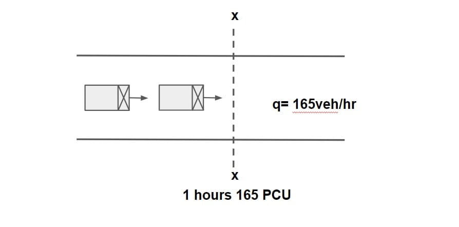
Traffic Volume (q)

Number of vehicle crossing the particular section of road is per unit time is called Traffic Volume. It is expressed in veh/day, veh/hr, veh/min.

PCU (Passenger Car Unit)

Under mixed traffic condition, It is difficult to find traffic volume, traffic density etc hence all class of vehicle are converted into a standard vehicle unit which is called PCU.

Class of Vehicle	PCU
Car, Tempo	1
Motar Cycle	0.5
Cycle Rickshaw	1.5
Bus, Truck	3
Horse Drawn Vehicle	4
Small Bullet Car	6
Large Bullet Car	8

\(PCU = \frac{\text{Speed Ratio}}{\text{Length Ratio}}\).

\(PCU = \frac{\frac{V_o}{V_i}}{\frac{L_o}{L_i}}\).

V_o and L_o = speed and length of standard vehicle.

Example: The free speed of a car on a 6 lane road is 120kmph, while that of a truck is 60kmph. The length of the car is 5m, where as the length of the truck is 10m. The PCU of the truck is ……

\(PCU =\frac{\frac{80}{40}}{\frac{5}{40}}=4\)

Measurements of Traffic Volume

Manual Method

In manual counts trained persons are posted at each lag of an intersection to count and record the number of trucks or buses, cars etc.

Mechanical Method 

• Radar (Radio Detection & Ranging)
• CCTV Cameras
• Magnetic Detector
• Pressure Sensitive Detectors

Presentation Of Traffic Volume Data  

Traffic Volume Data can be expressed in following different ways.

1. Annual Average Daily Traffic (AADT)
2. Annual Average Hourly Traffic (AAHT)
3. Annual Average Week Day Traffic (AAWT)
4. Average Daily Traffic (ADT)
5. Trend Chart
6. 30^th Highest Hourly Volume
7. Volume Flow Diagram at Intersection 
8. Variation Chart

Annual Average Daily Traffic (AADT)

AADT= \(\frac{\text{Total number of vehicles throughout a years}}{365}\) veh/day.

Annual Average Hourly Traffic (AAHT)

AAHT= \(\frac{\text{Total number of vehicles throughout a years}}{365×24}\) veh/hr.

AAHT= \(\frac{AADT}{24}\) veh/hr.

Annual Average Week Day Traffic (AAWT)

AAWT= \(\frac{\text{Total number of vehicles throughout week days}}{260}\) veh/day.

NOTE: AAWT>AADT, as on weekends traffic volume is considerably reduced.

Average Daily Traffic (ADT)

ADT= \(\frac{\text{Total number of vehicles throughout week}}{7}\) veh/day.

NOTE: ADT>AADT

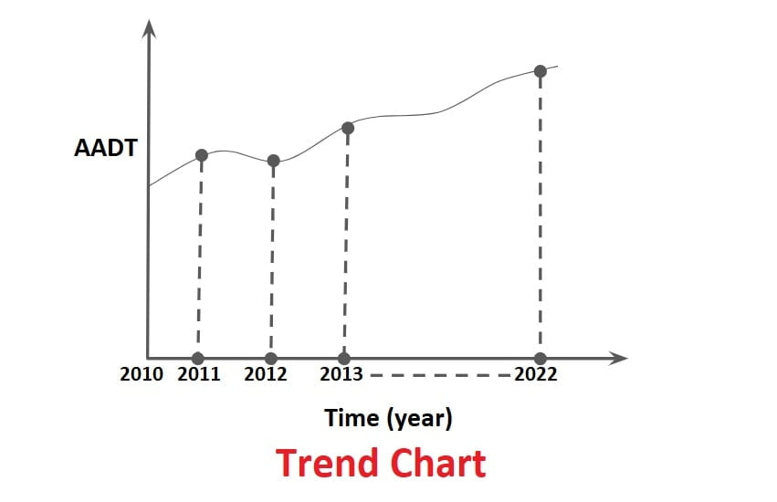
Trend Chart

1. Traffic volume data can be represented in form of Trend chart over period of years, which is useful in estimating the rate of growth of traffic that can be used for planning future expansion, design and regulation.
2. If from trend chart rate of growth of traffic volume is computed to be r%, then future traffic in given by

A=P(1+r)ⁿ

A= future traffic volume

P= present traffic volume

n= no of years.

Note: Average rate of growth of traffic is consider 5-7.5%.

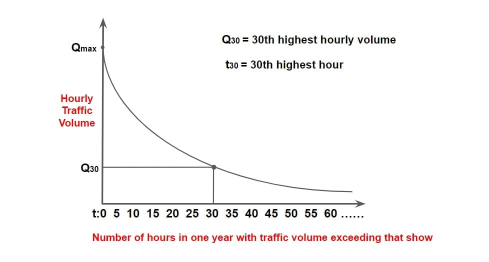
30^th Highest Hourly Volume

1. It has been observed that 30^th highest hourly volume gives a satisfactory results in terms of performance & it is economical in nature.
2. 30^th highest hourly volume is exceeded only 29 times in a years & all other traffic data will lie lesser than that.
3. IRC consider this traffic volume as Design Hourly Volume.

Volume Flow Diagram at Intersection 

• Volume flow diagram at intersection either drawn to a certain scale or indicating traffic volume can be used find the details of crossing & turning traffic.
• These data are required for design of Intersection.

 

Variation Chart

Variation charts shows the hourly, daily and seasonal variations. It helps in deciding the facilities and regulations needed during peak traffic hours.

NOTE:

Periodic Volume Count 

⇒In order to find certain traffic data, such as AADT, ADT etc. it is necessary to  count traffic for long duration of time(may be for years or months).

⇒Counting traffic for long duration of time, involves cost & effort which is not feasible practically.

⇒Hence to make reasonable estimate of certain traffic data concept of expansion factor can be used in Periodic Volume Count.

⇒In periodic volume count, expansion factors are used as follows.

1.Hourly Expansion Factor (HEF)

HEF= \(\frac{\text{Total traffic for a day}}{\text{Traffic for particular hour}}\)

2.Daily Expansion Factor (DEF)

DEF= \(\frac{\text{Total traffic for a week}}{\text{Traffic for particular day}}\)

3.Monthly Expansion Factor (MEF)

MEF= \(\frac{AADT}{ADT}\)

Peak Hour Factor (PHF)

It is defined as the ratio between the number of vehicles counted during the peak hour and four times the number of vehicles counted during the highest 15 consecutive minutes. Peak hour factor is a measure of the variation in demand during the peak hour.

\(PHF_{15} =\frac{\text{Hourly traffic volume}}{\frac{60}{15}\times V_{15}(max)}\).

\(PHF_{5} =\frac{\text{Hourly traffic volume}}{\frac{60}{5}\times V_{5}(max)}\).

V_₁5 = maximum number of vehicle during any 15 consecutive minutes

V₅ = maximum number of vehicle during any 5 consecutive minutes.

\(\frac{n}{60}\leq(PHF)_n\leq 1\).

---

---

  ⇒ Traffic Speed Studies  

Speed is the rate of travel expressed in kmph or m/s . Over a particular route, the actual speed of vehicle may vary. Speed of vehicle depends upon several factors such as geometric features, traffic conditions, time, place, driver and environment.

Types of Speed

1. Spot Speed
2. Average Speed
   1. Time Mean Speed
   2. Space Mean Speed
3. Journey Speed
4. Running Speed

Spot Speed

It is an instantaneous speed of vehicle at particular instant of time or section of road. It is measured by: Enoscope, Pressure Contact Tube, Loop Detector.

Average Speed

It is average speed of traffic calculate on the basic of spot speed of so many vehicle. It can be considered in two different ways.

1. Time Mean Speed
2. Space Mean Speed

Time Mean Speed

Arithmetic mean of spot speed of all vehicle is called Time Mean Speed.

\(V_t= \frac{V_1+V_2….+V_n}{n}\)

Space Mean Speed

It is harmonic mean of spot speed of all vehicle.

\(V_s= \frac{n}{\frac{1}{V_1}+\frac{1}{V_2}….+\frac{1}{V_n}}\)

Note: V_t>V_s

Journey Speed

Journey Speed =\(\frac{\text{length of journey}}{\text{time of journey}}\)

Running Speed

Running Speed =\(\frac{\text{length of journey}}{\text{Running time}}\)

Running Time = Journey Time – Delay 

Generally there are two type of speed studies carried out.

1. Spot Speed Study

2. Speed And Delay Study

---

1.Spot Speed Study

Spot speed studies cannot be used to find density because measurements are done at one point only. Spot speed studies are generally carried out for the following reasons:

• In accident studies
• To calculate the traffic capacity
• Planning of traffic regulations
• Decide the speed trends.

Representation Of Spot Speed Data

• Speed Distribution Table

• Frequency Distribution Curve

• Cumulative Speed of Vehicle

Speed Distribution Table 

From the spot speed data of the selected sample, frequency distribution tables are prepared for various speed range and no of vehicle in such range. The arithmetic mean is taken as average speed.

Example

Speed Rang (kmph)	No of Speed / Frequency Observed	% Frequency
0-10	5	1.25
10-20	8	2
20-30	10	2.5
30-40	17	4.25
40-50	30	7.5
50-60	46	11.5
60-70	200	50
70-80	52	13
80-90	32	8
	400

Frequency Distribution Curve

• Curve plotted between average values of each speed group on the x-axis and the frequency of vehicles in that group on y-axis is known as frequency distribution curve of the spot speed.
• A frequency distribution curve of spot speed is plotted with speed of vehicle or avg. value of each speed group of vehicle on the X- axis and the percentages of vehicle in that group on the Y- axis. This graph is called speed distribution curve.

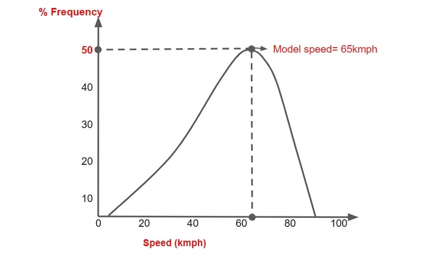
Model Speed

The speed at which greatest number of vehicle travels. It is the peak value of Frequency Distribution Curve.

Cumulative Speed of Vehicle

A graph is plotted between average value of each speed group on x-axis and cumulative percentage of vehicle travelled at or below different speeds on y-axis.

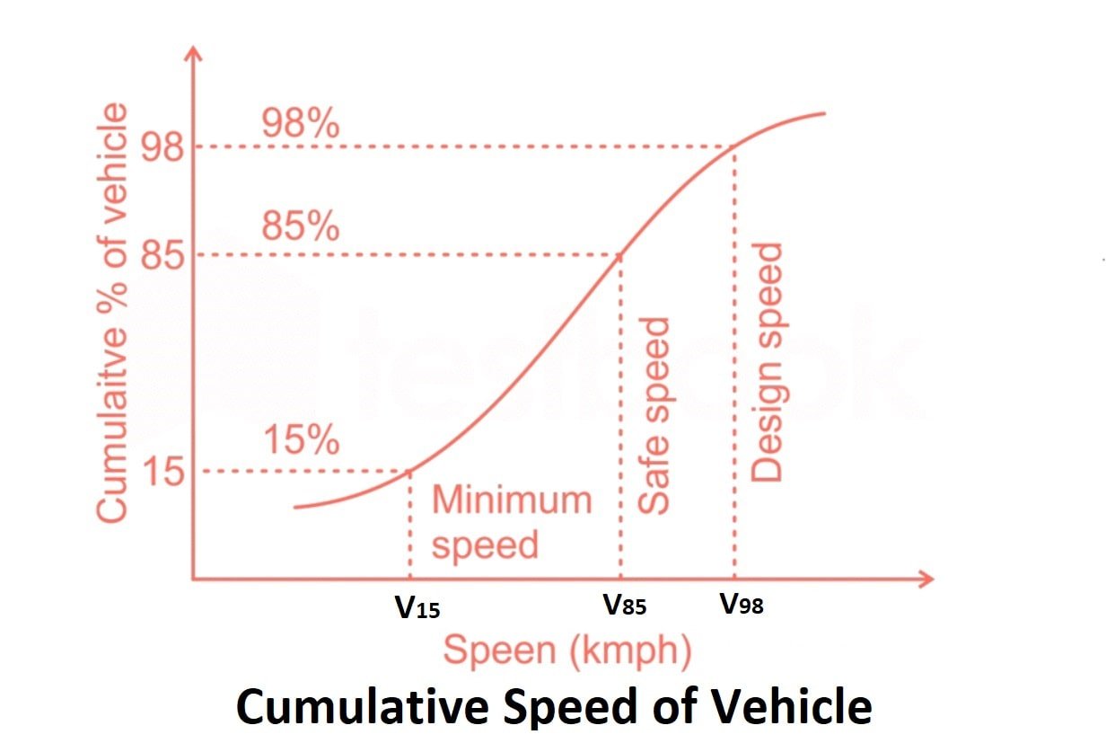
98th percentile speed

It is the speed at or below which 98% of vehicle are moving and only 2% exceeds this limit.

As per IRC this speed is considered as design speed for Geometric design.

85th percentile speed

It is the upper safe movement for vehicle movement.

This is adopted for safe speed limit.

15th Percentile Speed

It is the lower safe limit to avoid congestion.

Minimum speed on Major highway.

50th percentile speed

It is considered as median speed.

---

2. Speed And Delay Study

We know that spot speed study cannot give the density of traffic. Hence speed & delay studies are carried out over a long distance and hence it is possible to determine density of traffic. This study gives the running speeds, overall speeds, fluctuation in speed and delay between two stations.

There are various methods of carrying out speed and delay study.

• Floating Car Method
• License Plate Method
• Interview Technique
• Elevated Observations

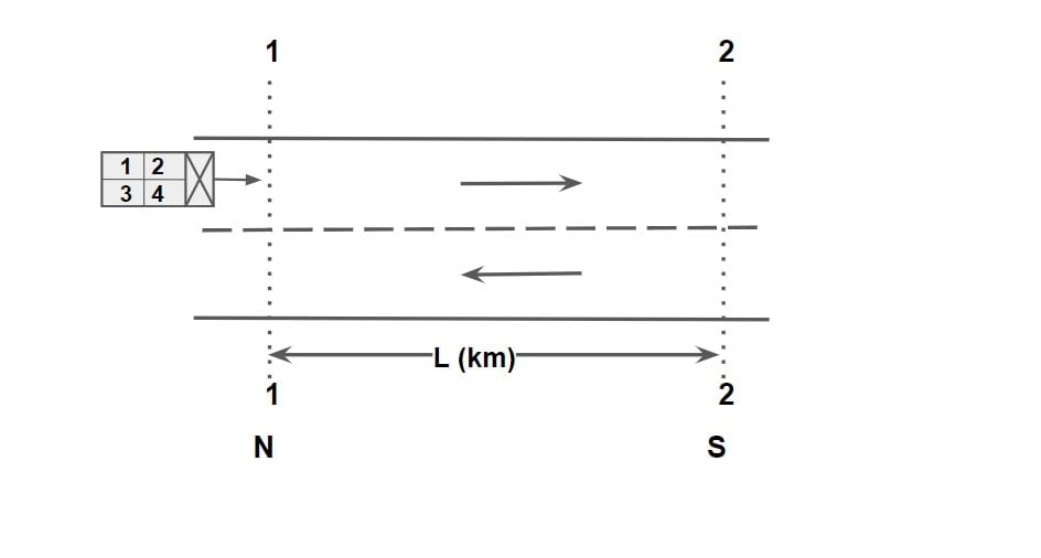
Floating Car Method

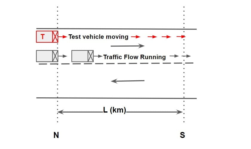
• This method is used only for two  lane two road. In this method a test vehicle is driven over a given length of road.
• Speed of text vehicle should be approximately same as speed of traffic.
• A group of four observers sitting in test vehicle records various details.

Observer 1: 1^st observer will be record total journey time and total cumulative delay time using 2 stop watches.

Observer 2: Location & Reasons for congestion will be noted by 2^nd observer.

Observer 3: Number of vehicle overtaking the test vehicles as well as overtaken by test vehicle will be noted by 3^rd observer.

Observer 4: 4^th observer counts total number of vehicles in opposite direction on adjacent length.

According to this Method

Traffic Flow (q):

\(q=\frac{n_a+n_y}{t_w+t_a}\)

Journey Time of Flow (\(\bar{t} \))

\(\bar{t}=t_w-\frac{n_y}{q}\)

where

t_w= Average journey time when the test vehicle is running with the flow.

t_a= Average journey time when the test vehicle is running against the flow.

n_y= Average no of vehicle overtaking the test vehicle – Average no of vehicle overtaken by the test vehicle.

n_y= overtaking – overtaken. {this can be +ve, -ve or even zero}

n_a= Average no of vehicle counted in the direction of stream when the test vehicle travels in the opposite direction. {n_a is measured by 4th observer of opposite direction of test vehicle}

Derivation Of Floating Car Method

Step.1 When test vehicle stop & all other vehicles is moving.

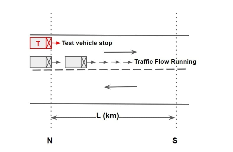
Traffic flow \(q=\frac{n_o}{T} \)

where

T= duration of study

n_o= number of vehicle overtaking the test vehicle

Step.2 When traffic is stop & test vehicle is moving.

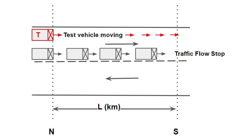
Traffic density \(K=\frac{n_s}{L} \)

n_s= KL= KV_TT

(∴L=V_TT)

n_s= KV_TT

where

n_s= number of vehicle overtaken by test vehicle

Step.3 When test vehicle is moving in the direction of flow & traffic is moving.

time of journey = t_w

n_y= Average no of vehicle overtaking the test vehicle – Average no of vehicle overtaken by the test vehicle.

n_o= number of vehicle overtaking the test vehicle = qt_w

n_s= number of vehicle overtaken by test vehicle = KL= KV_wt_w

(overtaking – overtaken)= n_y= qt_w – KV_wt_w

n_y= qt_w – KV_wt_w

n_y= qt_w – KL ……….(1)

Step.4 When test vehicle is moving in the opposite direction of flow & traffic is moving.

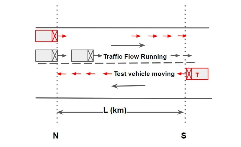time of journey = ta

n_a= Average no of vehicle counted in the direction of stream when the test vehicle travels in the opposite direction

n_a= qt_a + KV_at_a

n_a= qt_a + KL ……….(2)

add equation 1 & 2

ny = qtw – KL  +  na = qta + KL

ny+na = qtw + qta

Traffic Flow (q)

\(q=\frac{n_a+n_y}{t_w+t_a}\)

Journey Time of Flow (\(\bar{t} \))

from equation 1

n_y= qt_w – KL

K= q/v and L=vt

\(n_y=qt_w-\frac{q}{v}\times v\times t\).

\(n_y=qt_w-q\bar{t}\).

Journey time of flow

\(\bar{t}=t_w-\frac{n_y}{q}\)

---

---