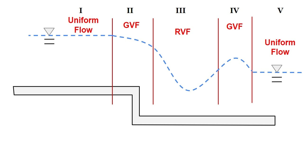
Gradually Varied Flow
♦ The gradually varied flow (GVF) is defined as steady non- uniform flow, where the depth of flow varies gradually from section to section along the length of the channel. (A steady non-uniform flow in a prismatic channel with gradual changes in its water surface elevation is termed as gradually varied flow (GVF).
♦ The back water produced by obstruction like dams or weirs across the river and the drawndown produced by a sudden drop in channel are examples of GVF.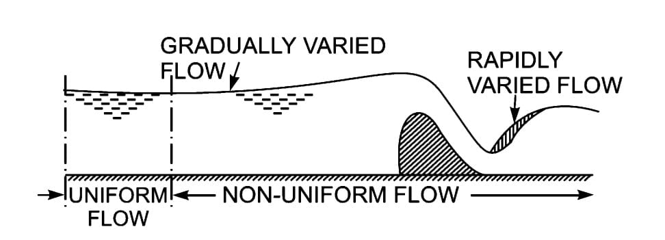
♦ In GVF, losses are negligible, the curvature of streamlines is negligible and the loss of energy is essentially due to boundary friction.
♦ In GVF Bed slope (So), water surface slope (Sw) and Energy slope (Sf) will all differ from each other.
♦ Almost all major hydraulic engineering activities in free surface flow involve the computation of GVF profiles.
Assumption In GVF
- Pressure distribution is hydrostatic because curvature of stream lines is small.
- Resistance to flow is given by Manning’s or Chezey’s equation with the slope taken as slope of energy line.
Manning’s Equation = \(\frac{1}{n}R^{2/3}S_f^{1/2}\)
Chezey’s Equation = \(CR^{1/2}S_f^{1/2}\)
- Channel bed slope is small i.e HGL will lie at free surface.
- There is no air entrainment.
- Velocity distribution is invariant i.e. kinetic energy correction factor, α= Constant
- Resistance coefficients (C & n) are constant with the depth.
- Channel is prismatic i.e. the channel has a constant alignment and its shape remains same over the reach of the channel under consideration.
Differential Equation of GVF 
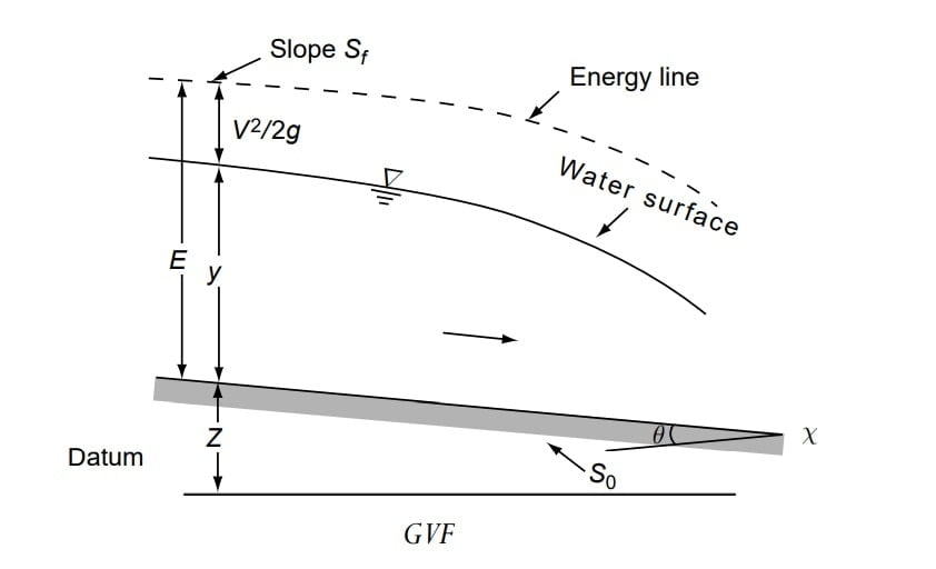
⇒ Consider the total energy H of a gradually varied flow in a channel of small slope and α = 1.0 as
H= Z + E
H= Z +y + v2/2g
where E = specific energy, v= Q/A
⇒ In general the water surface varies in the longitudinal (x) direction, the depth of flow and total energy are functions of x. Differentiating the above equation with respect to x
\(\frac{\mathrm{d} H}{\mathrm{d} x} =\frac{\mathrm{d} Z}{\mathrm{d} x}+\frac{\mathrm{d} y}{\mathrm{d} x}+\frac{d}{dx}(\frac{Q^{2}}{A^{2}\cdot 2g})\) ……..(1)
⇒ In above equation , the meaning of each term is as follows:
⇒ \(\frac{\mathrm{d} H}{\mathrm{d} x} \) represents the energy slope. Since the total energy of the flow always decreases in the direction of motion, it is common to consider the slope of the decreasing energy line as positive. Denoting it by Sf , we have
\(\frac{\mathrm{d} H}{\mathrm{d} x}= -S_f \)
⇒ \(\frac{\mathrm{d} Z}{\mathrm{d} x} \) denotes the bottom slope. It is common to consider the channel slope with bed elevations decreasing in the downstream direction as positive. Denoting it as S0, we have
\(\frac{\mathrm{d} Z}{\mathrm{d} x}= -S_o\)
⇒ \(\frac{\mathrm{d}y}{\mathrm{d} x} \) represents the water surface slope relative to the bottom of the channel.
⇒ \(\frac{d}{dx}(\frac{Q^{2}}{A^{2}\cdot 2g})\) = \(-\frac{Q^{2}}{gA^{3}}\frac{dA}{dy}\frac{dy}{dx}\)
since da/dy = T,
\(\frac{d}{dx}(\frac{Q^{2}}{A^{2}\cdot 2g})\) = \(-\frac{Q^{2}T}{gA^{3}}\frac{dy}{dx}\)
Equation 1 can now be rewritten as
\(-S_f=-S_o+\frac{dy}{dx}-\frac{Q^{2}T}{gA^{3}}\frac{dy}{dx}\)
Re-arranging
| \(\frac{dy}{dx}=\frac{S_o-S_f}{1-\frac{Q^{2}T}{gA^{3}}}\) |
This forms the basic differential equation of GVF and is also known as the dynamic equation of GVF. If a value of the kinetic-energy correction factor α greater than unity is to be used, Eq. would then read as
| \(\frac{dy}{dx}=\frac{S_o-S_f}{1-\alpha \frac{Q^{2}T}{gA^{3}}}\) |
Also,\(\frac{Q^{2}T}{gA^{3}}=Fr^{2}\)
| \(\frac{dy}{dx}=\frac{S_o-S_f}{1-Fr^{2}}\) |
Note:
1. If \(\frac{dy}{dx}\) >0 then the curved formed is called back water curve.
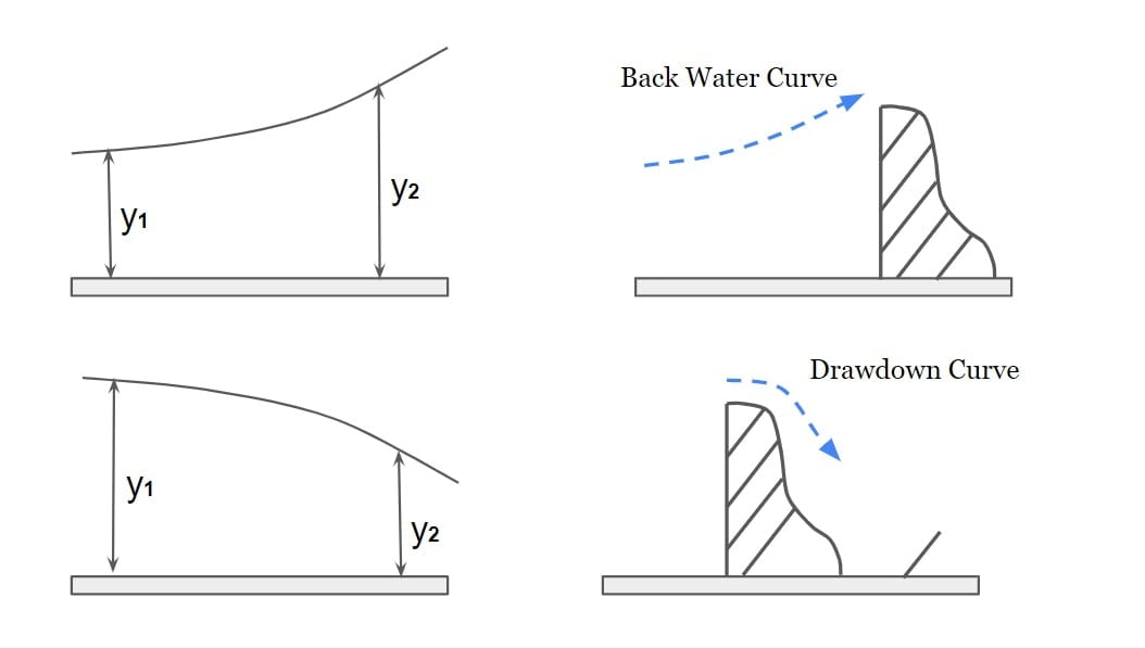
2. If \(\frac{dy}{dx}\) <0 then the curved formed is called draw down curve.
Differential Energy Equation
we know that, H=E+Z
Differentiating write to x
\(\frac{dH}{dx}=\frac{dE}{dx}+\frac{dz}{dx}\)
\(-S_f=-S_o+\frac{dE}{dx}\)
| \(\frac{dE}{dx}=S_o-S_f\) |
Classification Of Flow Profiles
⇒ (To study the GVF profile qualitatively we classify the flow under 12 group. The classification is important because it help to get overall understanding of how floe depth varies in a channel and also help to detect mistake in flow profile computation.)
⇒ A gradually varied flow profile is classified on the basis of channel slope and magnitude of flow depth ‘y’ in relation to ‘yn‘ & ‘yc‘.
⇒ The channel slope is classified on the basis of relative magnitude of normal depth ‘yo‘ and critical depth ‘yc‘.
Note: If channel section is wide rectangular (R= A/P & P=B+2y but for wide rectangular channel B>>2y so P = B). From Manning’s Equation
\(Q=\frac{A}{N}R^{2/3}S^{1/2} \).
\(Q=\frac{By}{N}(\frac{By}{B})^{2/3}S^{1/2} \).
\(Q=\frac{B}{N}(y)^{5/3}S^{1/2} \).
\(S^{1/2}=\frac{Q\cdot N}{B\cdot y^{5/3}}\).
assume constant c= \(c=\frac{Q\cdot N}{B}\)
\(S^{1/2}=\frac{c}{ y^{5/3}}\).
\(S=\frac{C}{ y^{10/3}}\).
hence
\(S_o=\frac{C}{ y_o^{10/3}}\).
\(S_c=\frac{C}{ y_c^{10/3}}\)
The slope of the channel can be classified as:
- There are 3 relations between yo and yc. (yo< yc), (yo> yc), (yo= yc).
- There are 2 relations when yo does not exists. (So<0), (So =0).
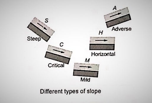
| S.No | Channel Category | Symbol | Characteristic condition | Remark |
| 1 | Mild slope | M | (yo> yc), (So<Sc) | Subcritical flow at normal depth |
| 2 | Steep slope | S | (yo< yc), (So>Sc) | Supercritical flow at normal depth |
| 3 | Critical slope | C | (yo= yc), (So=Sc) | Critical flow at normal depth |
| 4 | Horizontal slope | H | (yo= ∞), (So=0) | Cannot sustain uniform flow |
| 5 | Adverse slope | A | (So<0) | Cannot sustain uniform flow |
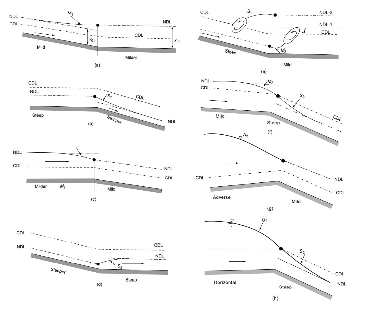
⇒ Flow profile associated with these channel slopes are designated as M, S, C, H, A for respective slopes and the space above the channel bed can be decided into three zone depending upon the relative magnitude of y, yo, yc.
⇒ The space above both CDL and NDL is designated as Zone-I. (y>yo, yc ).
⇒ The space between CDL and NDL is designated as Zone-II. (yo/ yc < y <yo/ yc ).
⇒ The space between the channel bed and NDL/CDL (whichever is lower) is designated as Zone-III. (0≤ y <yo/ yc ).
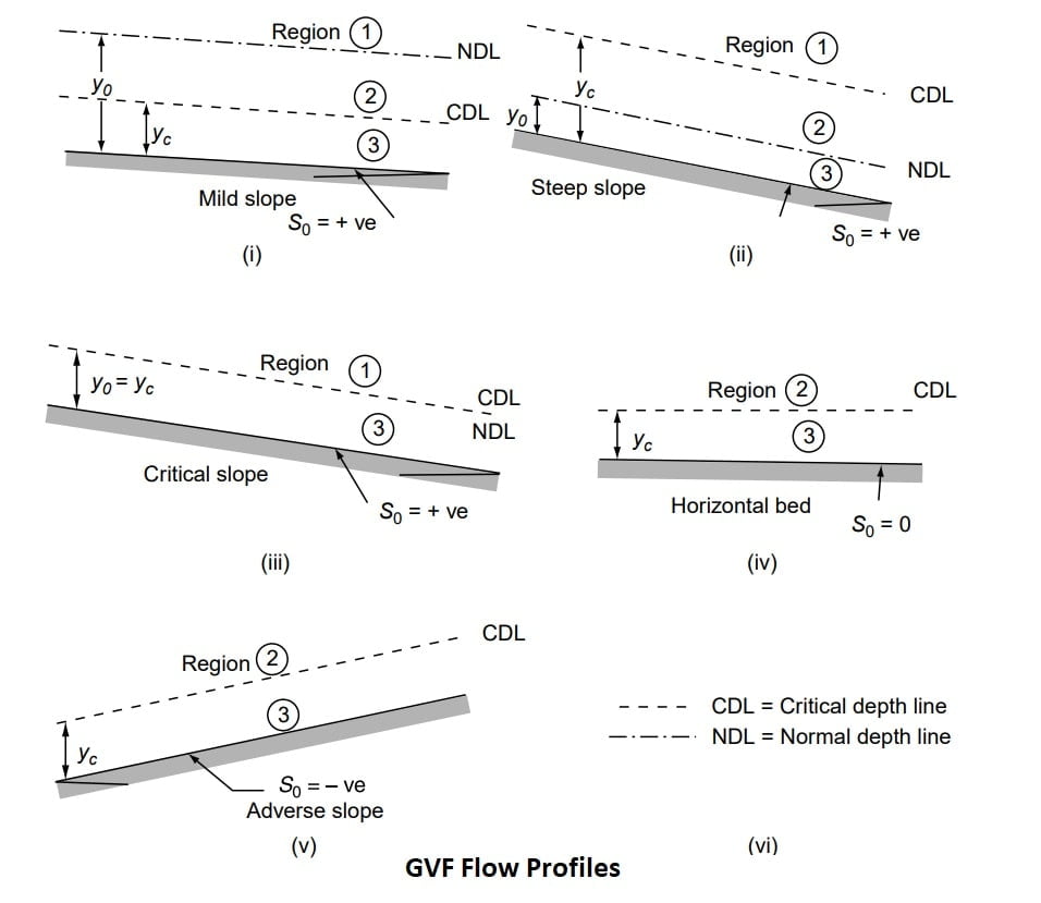
⇒ Classification of flow profile is done based in the slope of channel and the region of flow. Hence, we can have 12 different types of flow profiles.
| Channel | Region | Condition | Type |
| Mild slope | 1 2 3 | y>yo>yc yo>y>yc yo>yc>y | M1 M2 M3 |
| Steep slope | 1 2 3 | y>yc>yo yc>y>yo yc>yo>y | S1 S2 S3 |
| Critical slope | 1 3 | y>yo=yc y<yo=yc | C1 C3 |
| Horizontal slope | 2 3 | y>yc y>yc | H2 H3 |
| Adverse slope | 2 3 | y>yc y>yc | A2 A3 |
⇒ Classification of flow profile is important because it gives an understanding of how the flow depth varies in the channel.
Following Point Must Be Noted Before Studding the Characteristic of Flow Profile.
⇒ Head loss increases with increase in velocity & decrease in depth.
hL ∝ v ∝ (1/y)
⇒ If energy line is parallel to the channel bed, i.e slope of energy line is equal to the bed slope, flow will takes place at normal depth.
Sf = So ⇒ y = yn
So – Sf =0
⇒ If slope of energy line is greater than the bed slope, flow will take place at depth less then the normal depth.
Sf > So ⇒ y < yn
So – Sf <0
⇒ If slope of energy line is less than the bed slope, flow will take place at depth greater then the normal depth.
Sf < So ⇒ y > yn
So – Sf >0
⇒ If So= 0 then So – Sf <0. (horizontal slope)
⇒ If So<0 then So – Sf <0. (adverse slope)
⇒ If y>yc then Fr <1. (Sub critical flow) {1-Fr2 >0}
⇒ If y<yc then Fr>1.(Super critical flow) {1-Fr2 <0}
⇒ If y=yc then Fr =1. {1-Fr2 = 0}
Important Point
\(\frac{dy}{dx}=\frac{S_o-S_f}{1-Fr^{2}} = \frac{ numerator(N)}{denominator(D)}\)
1. \(\frac{dy}{dx}\) is positive if both numerator and denominator both are positive or negative.
Case.1
\(\frac{N}{D}=\frac{+}{+}=+\)
For N = +ve, y > yn
For D =+ve, y > yc
so y > yn & yc ⇒ Region 1 (M1, S1, ….)
Case.2
\(\frac{N}{D}=\frac{-}{-}=+\)
For N = -ve, y < yn
For D =-ve, y < yc
so y < yn & yc ⇒ Region 3 (M3, S3, ….)
Rule.1 ⇒ Thus in region 1 & 3 flow profile always increase in the direction of flow.
2. \(\frac{dy}{dx}\) is negative if
Case.1
\(\frac{N}{D}=\frac{+}{-}=-\)
For N = +ve, y > yn
For D =-ve, y < yc
so yc >y > yn ⇒ Region 2 (S2, ….)
Case.2
\(\frac{N}{D}=\frac{-}{+}=+\)
For N = -ve, y < yn
For D =+ve, y > yc
so yn >y > yc ⇒ Region 2 (M2, ….)
Rule.2 ⇒ Thus in region 2 flow profile always decrease in the direction of flow.
3.
If y →yn
then Sf → So
\(\frac{dy}{dx}=\frac{S_o-S_f}{1-Fr^{2}} = 0\)
Rule.3 ⇒ Thus water surface profile approach normal depth asymptotically if depth of flow approaches to normal depth of flow.
4.
If y →yc
then Fr →1
\(\frac{dy}{dx}=\frac{S_o-S_f}{1-Fr^{2}} = \infty\)
θ=90°
Rule.4 ⇒ Thus water surface profile approach critical depth line vertically if depth of flow approaches to critical depth vertically.
Note: Under this situation, flow profile will have very steep slope and hence curvature of flow profile will large and it can not be treated as GVF. Due to large curvature, normal acceleration can not be assumed to be zero and hydrostatic condition will not be valid. Thus over here assumption of hydrostatic condition will be neglected.
5.
If y →∞
then Fr →0
Sf →0
\(\frac{dy}{dx}=\frac{S_o-S_f}{1-Fr^{2}} = S_o\)
Rule.5 ⇒ Surface profile become horizontal as flow depth becomes large.
6.
If y →0
\(\frac{dy}{dx}=\frac{S_o-S_f}{1-Fr^{2}} = \infty\)
θ=90°
Rule.6 ⇒ Surface profile meets the bed vertically if depth of flow reduces to zero.
Note: It can be show that for wide rectangular channel \(\frac{dy}{dx}=\frac{gy^{3}(S_oy^{10/3}-q^{2}n^{2})}{y^{10/3}(gy^{3}-q^{2})}\) from the above relation we can observe that as y → 0, \(\frac{dy}{dx}\rightarrow \infty\), i.e water surface profile become vertical as the flow depth tends to zero.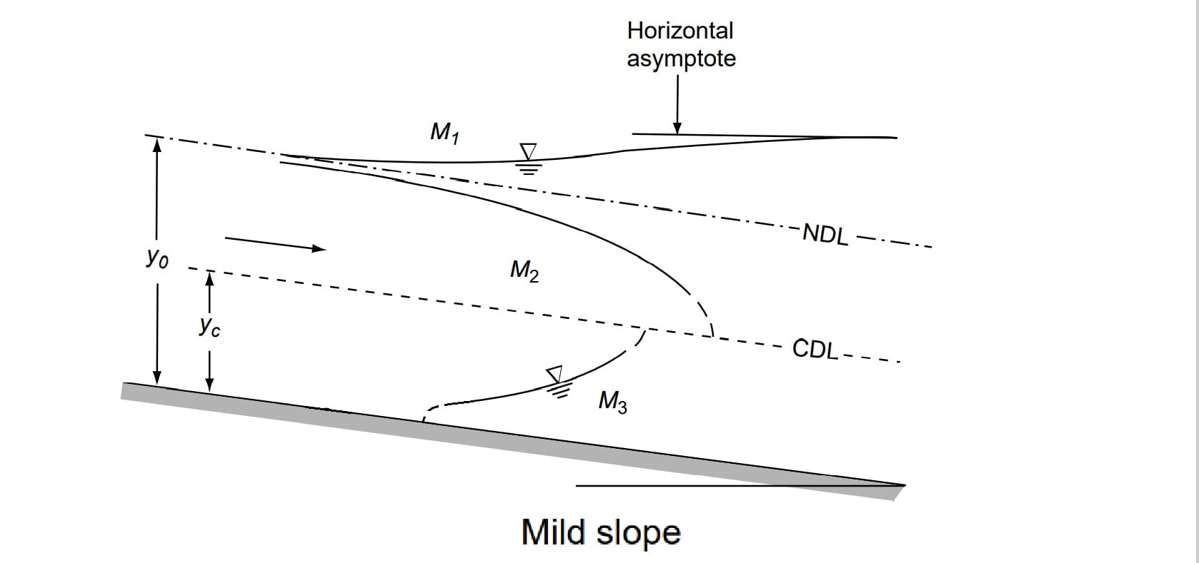
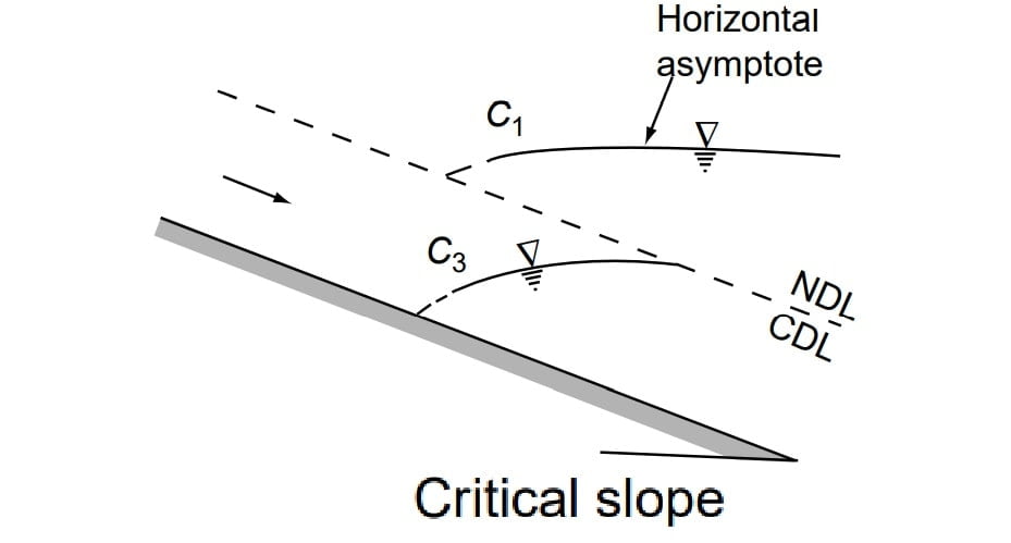
Note: C1 & C3 profile will be straight line if chezy equation is use to obtaining dy/dx and it could be curved if manning’s equation is used for obtaining dy/dx however the difference is insignigicant.
Practical Cases of GVF Profile
(A) Type-M Profiles
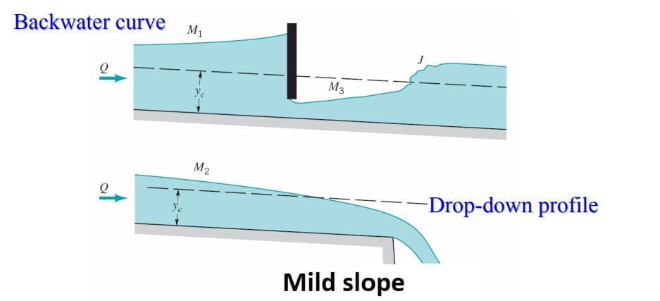
M1 Profile
The most common of all GVF profiles is the M1 type, which is a subcritical flow condition. Obstructions to flow, such as weirs, dams, control structures and natural features, such as bends, produce M1 backwater curves. These extend to several kilometres upstream before merging with the normal depth.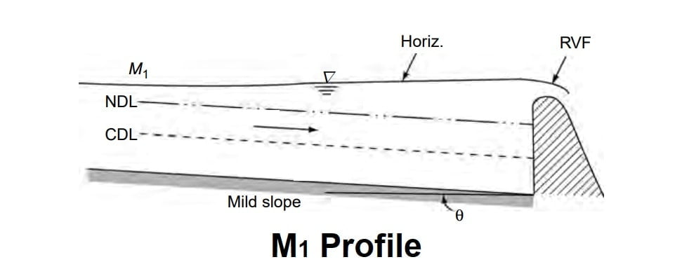
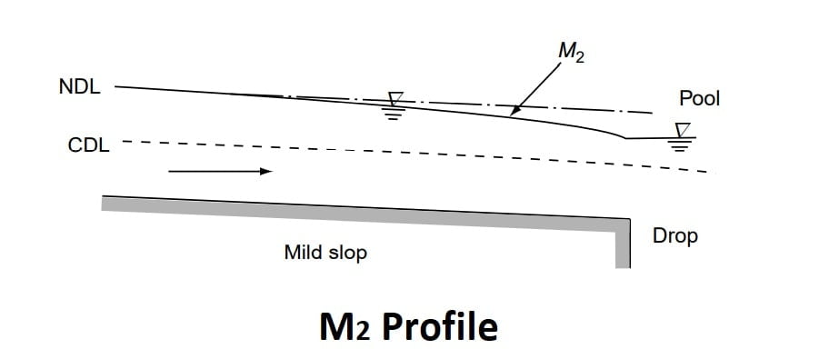
M2 Profile
The M2 profiles occur at a sudden drop in the bed of the channel, at constriction type of transitions and at the canal outlet into pools.
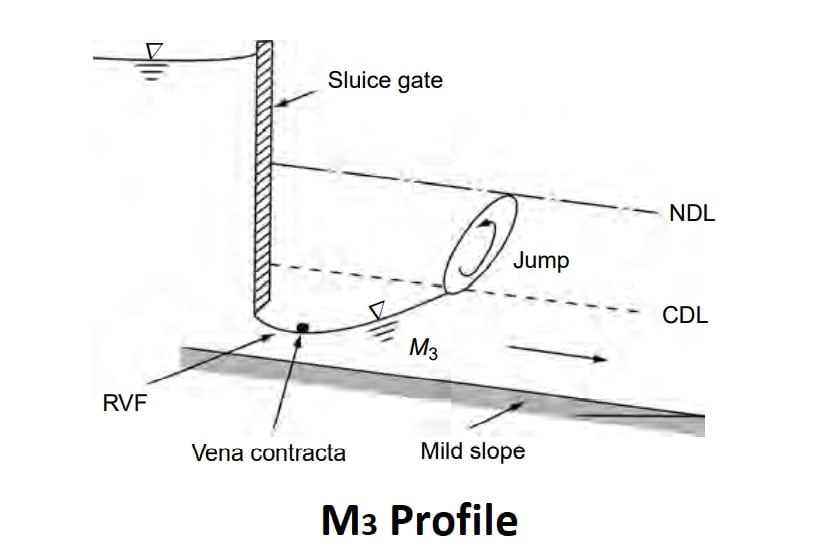
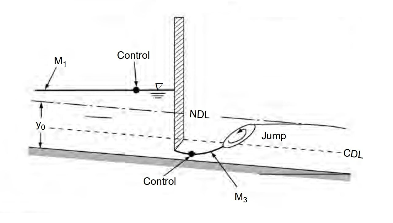
M3 Profile
Where a supercritical stream enters a mild-slope channel, the M3 type of profile occurs. The flow leading from a spillway or a sluice gate to a mild slope forms a typical example. The beginning of the M3 curve is usually followed by a small stretch of rapidly-varied flow and the down stream is generally terminated by a hydraulic jump. Compared to M1 and M2 profiles, M3 curves are of relatively short length.
Note:
- M3 profile is always flowed by a hydraulic jump.
- M3 presided by a small reach of RVF.
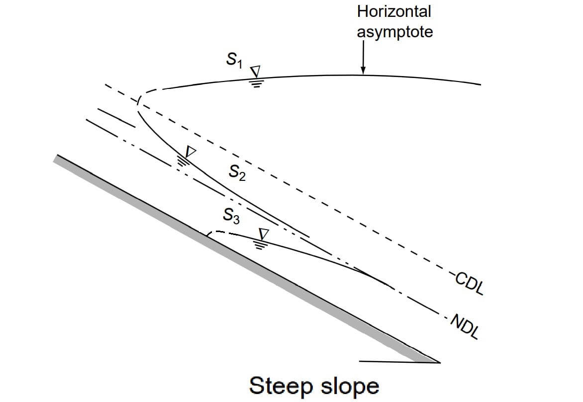
(B) Type-S Profiles
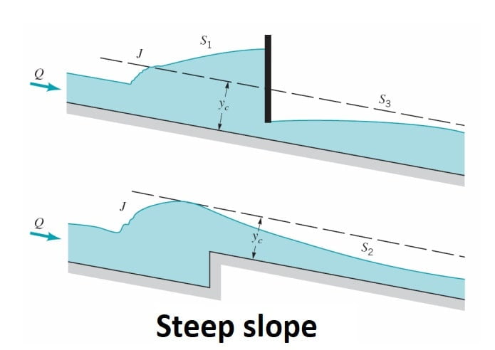
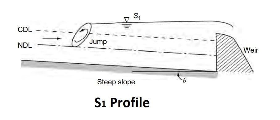
S1 Profile
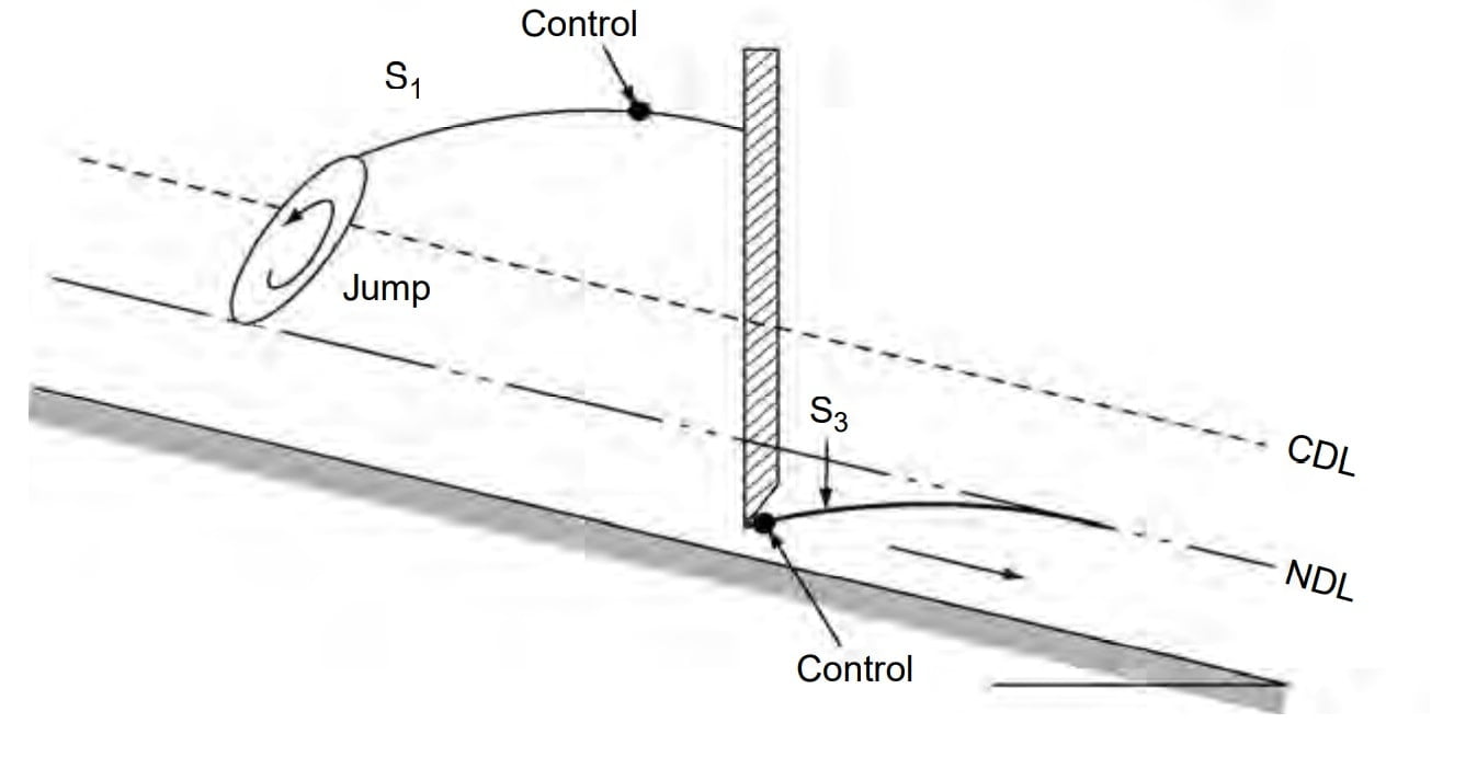
The S1 profile is produced when the flow from a steep channel is terminated by a deep pool created by an obstruction, such as a weir or dam. At the beginning of the curve, the flow changes from the normal depth (supercritical flow) to subcritical flow through a hydraulic jump. The profiles extend downstream with a positive water surface slope to reach a horizontal asymptote at the pool elevation.
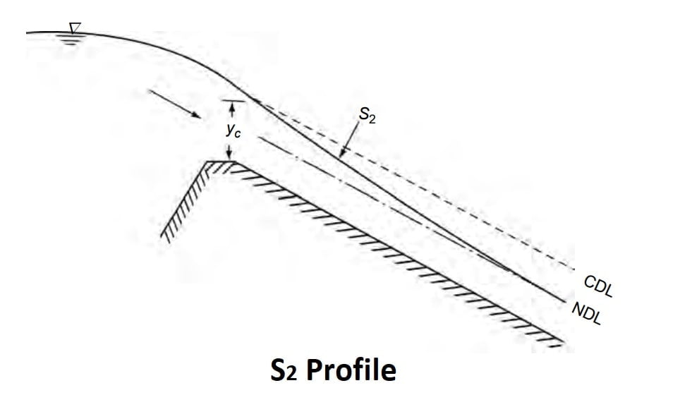
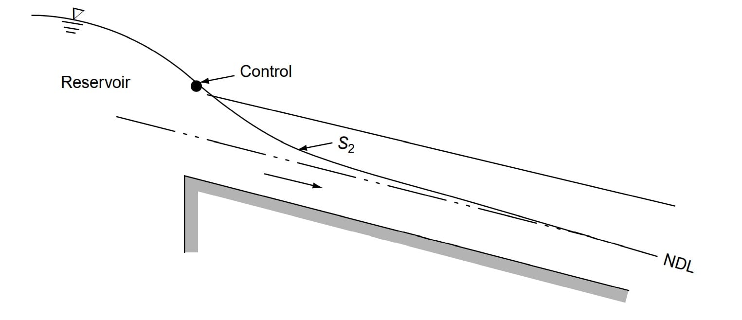
S2 Profile
Profiles of the S2 type occur at the entrance region of a steep channel leading from
a reservoir and at a break of grade from mild slopes to steep slope (Fig.). Generally S2 profiles are of short length..
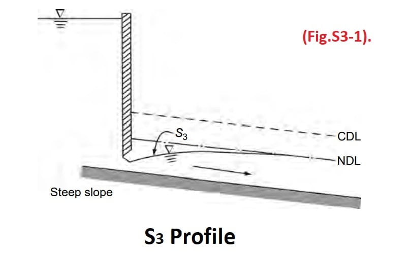
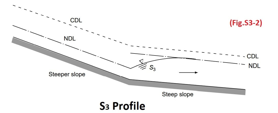
S3 Profile
Free flow from a sluice gate with a steep slope on its downstream is of the S3 type (Fig.S3-1). The S3 curve also results when a flow exists from a steeper slope to a less steep slope (Fig.S3-2).
(C) Type-C Profiles
C1 and C3 profiles are very rare and are highly unstable.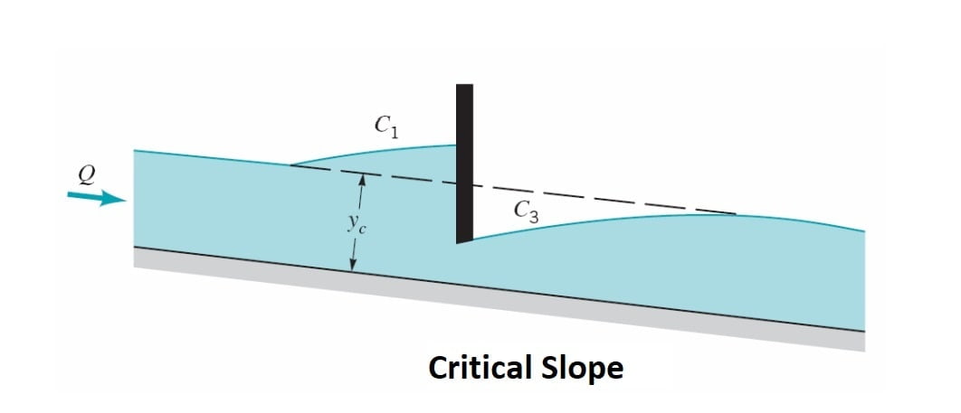
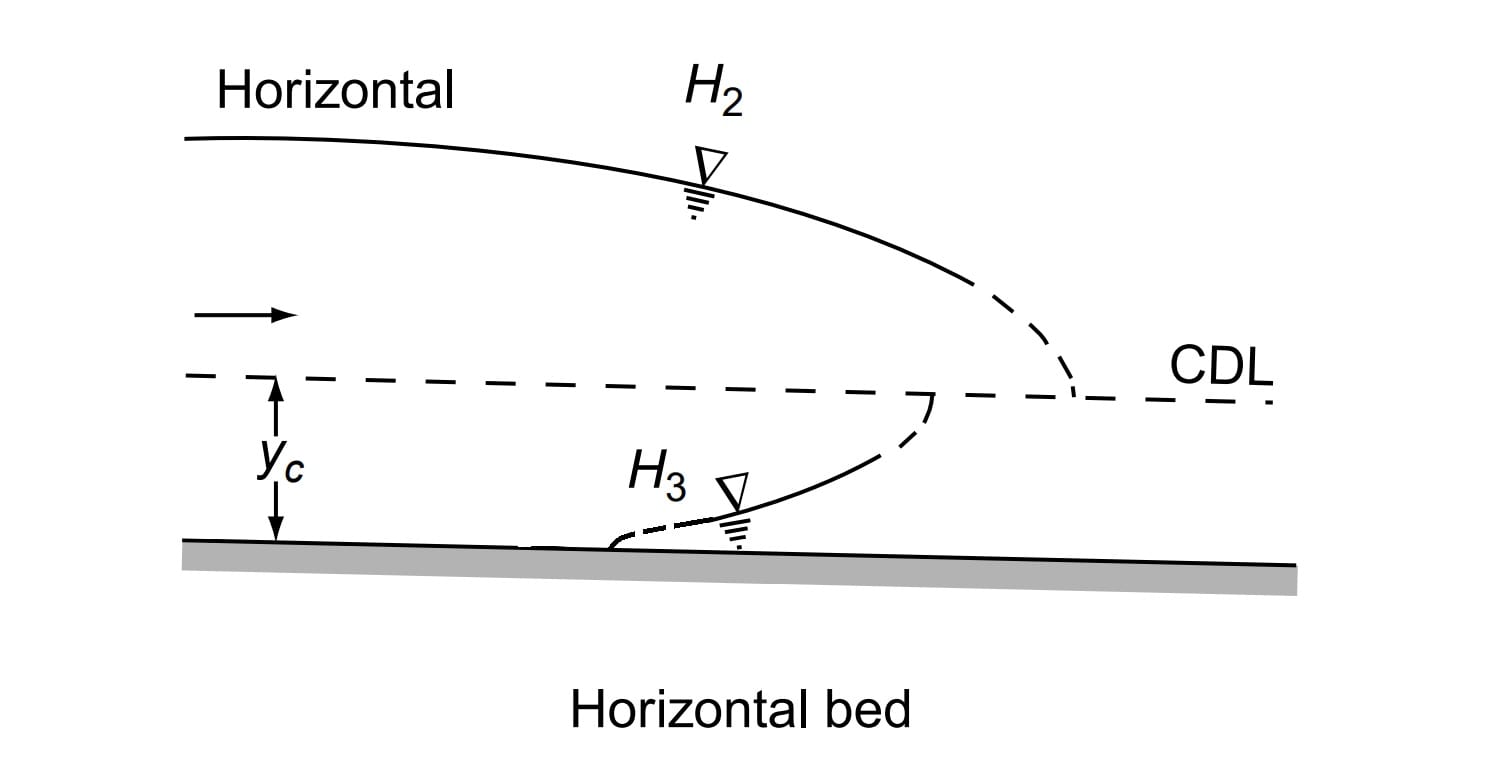
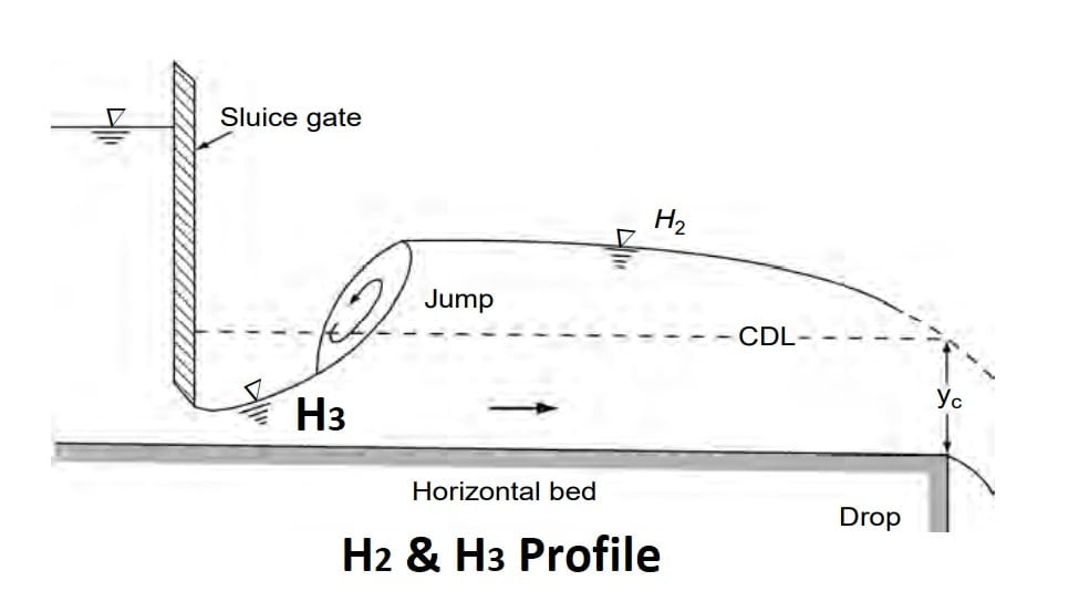
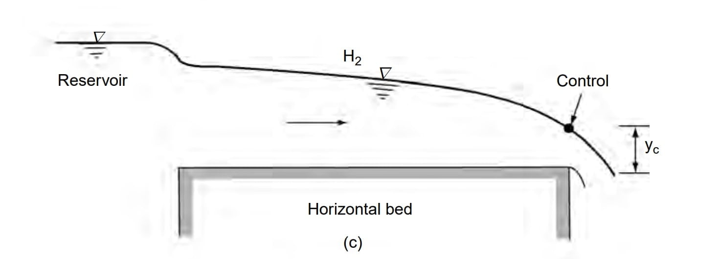
(D) Type-H Profiles
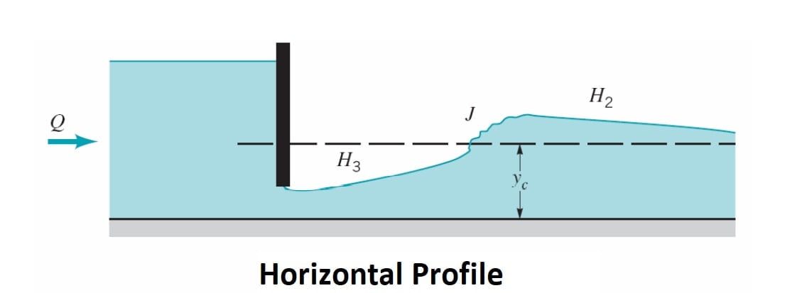
A horizontal channel can be considered as the lower limit reached by a mild slope as its bed slope becomes flatter. It is obvious that there is no region 1 for a horizontal channel as y0 = ∞. The H2 and H3 profiles are similar to M2 and M3 profiles respectively [Fig. ]. However, the H2 curve has a horizontal asymptote.
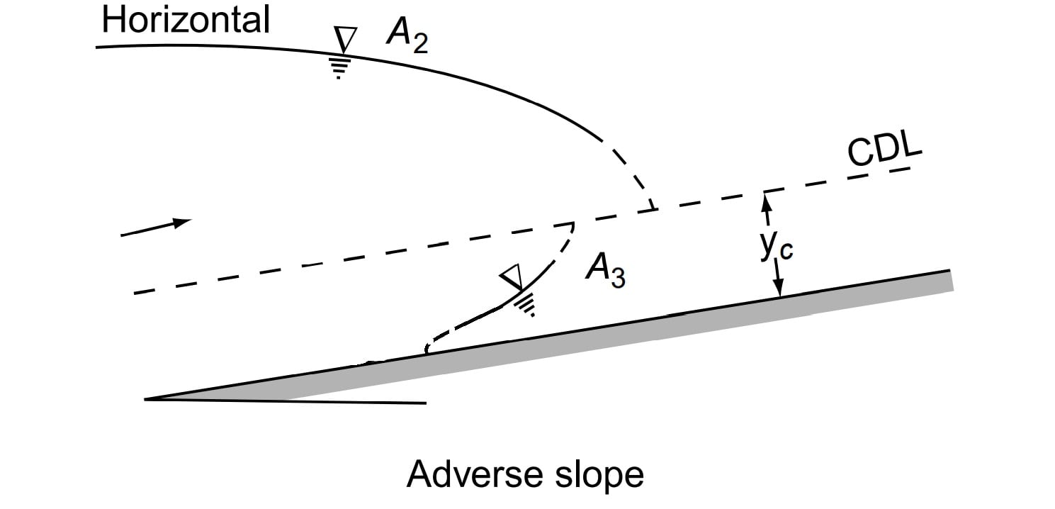
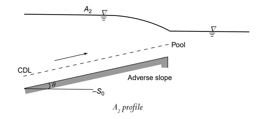
(E) Type-A Profiles
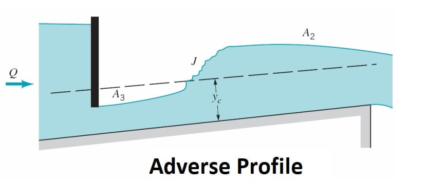
Adverse slopes are rather rare and A2 and A3 curves are similar to H2 and H3 curves respectively (Fig. ). These profiles are of very short length.
Note: M3, H3, A3, followed by hydraulic jump and S1 profiles is preceded by hydraulic jump.
Control Section
⇒ A control section is defined as a section in which a fixed relationship exists between the discharge and depth of flow. Weirs, spillways, sluice gates, are some typical examples of structures which give rise to control sections.
⇒ Control section is a point where calculation of GVF profile starts.
⇒ It proceed upstream in case of subcritical flow & downstream in case of supercritical flow hence Supercritical flow has u/s control section & Subcritical flow has d/s control section.
⇒ If y>yc then Fr <1. (Sub critical flow)
⇒ If y<yc then Fr>1.(Super critical flow)
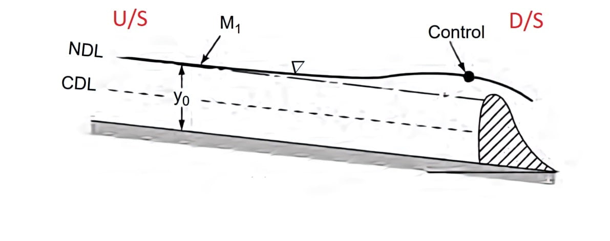
In M1 profile, y>yc then Fr <1.Flow is Sub-critical flow. So subcritical flow has d/s control section.
In M1 profile y>yc then Fr <1, Flow is Sub-critical flow. So subcritical flow has d/s control section.
In M3 profile y<yc then Fr >1, Flow is Super-critical flow. So supercritical flow has u/s control section
In S1 profile y>yc then Fr <1, Flow is Sub-critical flow. So subcritical flow has d/s control section.
In S3 profile y<yc then Fr >1, Flow is Super-critical flow. So supercritical flow has u/s control section
In S2 profile y<yc then Fr >1, Flow is Super-critical flow. So supercritical flow has u/s control section.
In H2 profile y>yc then Fr <1, Flow is Sub-critical flow. So subcritical flow has d/s control section.
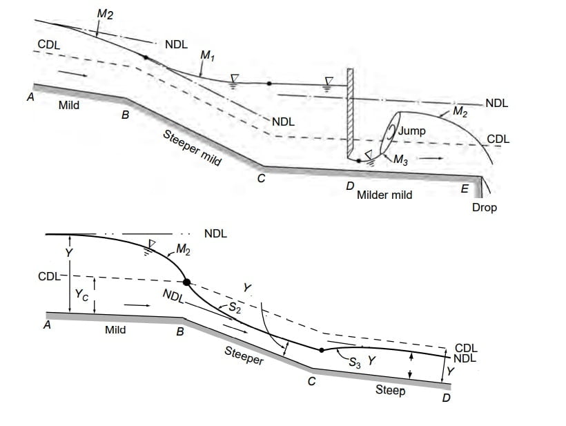
Break In Grade
⇒ When two channel section have different bed slope the section is called break in grade.
⇒ Following points must be noted for analysis of flow profile.
- For sub critical flow → control section is downstream.
- For super critical flow → control section is upstream.
- Draw CDL & NDL for different slope.
- CDL is at a constant height above the channel bed in different slopes as yc is independent of bed slope of channel.
- Match the NDL for various type of flow.
- When a supercritical flow meets a subcritical flow, it creates a hydraulic jump.
Gradually Varied Flow Computation
Almost all major hydraulic engineering activities in free surface flow involve the computation of GVF profiles.
The various available procedure for computing GVF profiles can be classified as
- Direct integration – Chow’s Method
- Numerical Method – Direct step Method
- Graphical Method.
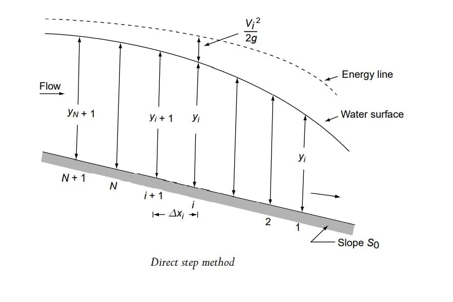
Direct Step Method
This method is the simplest & suitable foe prismatic channels.
\(\frac{dE}{dx}=S_o-S_f\)
writing above equation in finite difference form
\(\frac{\Delta E}{\Delta x}=S_o-\bar{S_f}\)
\(\Delta x=\frac{\Delta E}{S_o-\bar{S_f}}\)
where, \(\bar{S_f}\) = average friction slope in reach Δx
\(x_2-x_1=\frac{E_2-E_1}{S_o-\frac{1}{2}(Sf_1+Sf_2)}\)
Note: In order to calculate average slope of TEL ‘Sf’ following procedure can also be adopted.
\(y_{avg} = \frac{y_1+y_2}{2}\)
Q=Av
Q= \(B\cdot y_{avg}\frac{1}{N}\cdot R_{avg}^{2/3}\bar{S_f}^{1/2}\)
Procedure For Computation of GVF Profiles
Finding out the value of Δx.
Let it is to be required to find the water surface profile between two sections ‘1’ & ‘N+1’, where the depth of flow are y1 & yN+1 respectively.
Channel reach is divided into N parts of known depth.
Our requirement is to find distance Δxi
Now between two section ‘3’ and ‘4’
ΔE= \(\Delta (y+\frac{v^{2}}{2g})\)
ΔE= \(\Delta (y+\frac{Q^{2}}{2gA^{2}})\)
ΔE= \(y_{i+1}-y_i+\frac{Q^{2}}{2gA_{i+1}^{2}}-\frac{Q^{2}}{2gA_i^{2}}\)
\(\bar{S_f}=\frac{1}{2}(S_{fi+1}-S_{fi})\)
Q= Av= A\(\frac{1}{N}R^{2/3}S^{1/2}\)
\(S=\frac{Q^{2}N^{2}}{A^{2}R^{4/3}}\)
\(\bar{S_f}=\frac{1}{2}Q^{2}N^{2}(\frac{1}{A_{i+1}^{2}R_{i+1}^{4/3}}+\frac{1}{A_{i}^{2}R_{i}^{4/3}})\)
Calculate \(\Delta x_i=\frac{\Delta E}{S_o-\bar{S_f}}\)
The sequential evolution of Δxi starting from i=1 to N will be done & summation of these Δxi would give the length of GVF.
Question : Determine the length of Backwater curve caused by afflux of 1.5m in rectangular channel of width 50m and depth 2m. Assume So= 1/2000 & n= 0.03
Solution:
Afflux = 1.5m
y1=2m
y2= 2+1.5= 3.5m
At section 1
Q= A1v1
Q= A\(\frac{1}{N}R^{2/3}S_0^{1/2}\)
R= A/P
A1= 50*2 =100
P1 = 50+2+2=54
R1 = 100/54 =1.851
Q = 100×(1/0.03)×(1.851)2/3×(1/2000)1/2
Q = 112.4 m3/sec
\(E_1= y_1+\frac{Q^{2}}{2gA_1^{2}}\)
E1 = 2+ \(\frac{112.4^{2}}{2\times 9.81\times 100^{2} }\)
E1 = 2.064m
At section 2
Q= A2v2
Q= A\(\frac{1}{N}R^{2/3}S_f^{1/2}\)
R= A/P
A2= 50*3.5 =175
P2 = 50+2×3.5=57
R2 = 175/57 =3.070
\(E_2= y_2+\frac{Q^{2}}{2gA_2^{2}}\)
E2 =3.5+ \(\frac{112.4^{2}}{2\times 9.81\times 175^{2} }\)
E2 = 3.52m
yavg= (y1+y2)/2 = 5.5/2 =2.75m
Ravg = (1.851+ 3.070)/2 = 2.461m
Q= Av
Q= A\(\frac{1}{N}R^{2/3}\bar{S_f}^{1/2}\)
112.4 = (50×2.75)(1/0.03)(2.461)2/3×\(\bar{S_f}^{1/2}\)
0.0134538 =\(\bar{S_f}^{1/2}\)
\(\bar{S_f}\) =0.0001810
\(\bar{S_f}\) =1/5524
\(\Delta x=\frac{E_2-E_1}{S_o-\bar{S_f}}\)
\(\Delta x=\frac{3.52-2.064}{\frac{1}{2000}-\frac{1}{5524}}\)
\(\Delta x=4564.64m\) = 4.56Km
Question: A widen rectangular channel carries a discharge of 8 m3/sec-m width. The channel has a bed slope 0.004 and n= 0.015. At a certain section of channel the flow depth is 1m.
- What GVF profile from this section.
- At what distance from this section the flow depth will be 0.9m (use direct step method employing single step)
Solution:
q=8m3/s-m
n=0.015
y=1m
So=0.004
wide rectangular channel (R≈yn)
\(y_c=(\frac{q^{2}}{g})^{1/3}\).
\(y_c=(\frac{8^{2}}{9.81})^{1/3}\)= 1.868m
Q=Av
q= yn×v
q = yn× (1/n)R2/3 S1/2
8 = yn× (1/0.015)yn2/3 0.0041/2
yn =1.468m
yn <yc ⇒ channel is steep.
y < yn <yc ⇒ GVF is S3.
yavg= (y1+y2)/2 = (1+0.9)/2 = 0.95m
Ravg = yavg
q= yavg×v
q= yavg× (1/n)R2/3 Sf1/2
8 = 0.95× (1/0.015)0.952/3 (Sf)1/2
\(\bar{S_f}\) =0.017
ΔE=E2-E1 = \((y_2+\frac{q^{2}}{2gy_2^{2}})-(y_1+\frac{q^{2}}{2gy_1^{2}})\)
ΔE= \((1+\frac{8^{2}}{29.812^{2}})-(y_1+\frac{q^{2}}{2gy_1^{2}})\)
ΔE= \((1+\frac{8^{2}}{2\times 9.81\times 2^{2}})-(0.9+\frac{8^{2}}{2\times 9.81\times0.9^{2}})\)= -0.665m
\(\Delta x=\frac{E_2-E_1}{S_o-\bar{S_f}}\)
\(\Delta x=\frac{-0.665}{0.004-0.017}\)
\(\Delta x=51.15m\) = 51.15m