Traffic Engineering

The basic objective of traffic engineering is to achieve free & rapid flow of traffic with least no of accidents. For this various studies are carried out. These studies are divided into

1. Traffic Characteristics
2. Traffic Studies and Analysis
3. Traffic Control Regulation

---

---

  1. Traffic Characteristics  

In traffic characteristics, we generally study

1. Road User Characteristics
2. Vehicular Characteristics
3. Breaking Characteristics

A. Road User Characteristics

Factor Affecting Road User Characteristics:

1. Physical: Vision, hearing, strength and General reaction to traffic situation.
2. Mental: Knowledge, skill, experience, intelligence.
3. Psychological: Fear, anger, impatience, maturity.
4. Environmental: Facilities to the traffic, atmospheric condition and locality.

Vision

\(vision = \frac{x}{y}= \frac{\text{Actual distance}}{\text{Requried distance}}\)

6/6 Vision / Normal Vision: It is an ability of a person to recognize a letter of size 8.5 mm at a distance of 6m.

6/9 Vision / Poor Vision: This vision is poorer then normal vision because he can recognize at a distance of 6 m but a Normal person can recognize at a distance of 9 m.

NOTE: Concept of 6/6 and 6/9 vision used to design of location of sign board.

B. Vehicular Characteristics

In vehicular characteristics, we generally study

1. Dimension
2. Weight of Loaded Vehicle
3. Power of Vehicle
4. Speed of Vehicle

Dimension

• Length of vehicle affects turning radius, extra widening, parking design etc. (Maximum length 18 meter)
• Width of vehicle affects lane width, shoulder width and parking design.  (Maximum width 2.44 meter)
• Height of vehicle affects height of bridges, height of pole, etc. (Maximum height 4.75 meter)

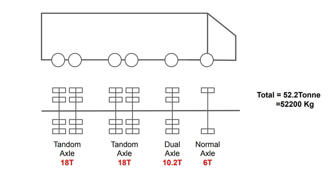
Weight of Loaded Vehicle

Weight affects design gradient & thickness of pavement.

Power of Vehicle

It affects the limiting & design value of the gradient.

Speed of Vehicle

It affects all geometrical elements & traffic control devices.

C. Breaking Characteristics

At least two of the following three parameters are needed during the breaking test in order to determine skid resistance of pavement.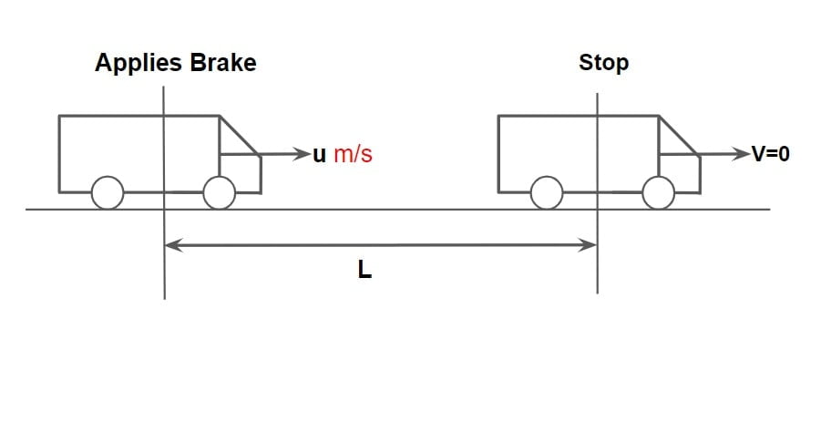

• initial speed (u m/s)
• length of skid distance (L meter)
• Time of break application (t sec)

⇒ Retardation

v-u = at

(v=o)

-u= at

-a= u/t

Retardation =\(\frac{\text{initial speed}}{\text{time}}\) 

⇒ Skid Distance

\(L=ut+\frac{1}{2}at^{2}\).

\(a=\frac{-u}{t}\).

\(L=ut+\frac{1}{2}\frac{-u\cdot t^{2}}{t}\).

\(L=ut-\frac{1}{2}ut\).

\(L=\frac{1}{2}ut\).

\(\text{Skid distance} = \frac{1}{2}\times \text{initial speed}\times \text{time}\).

⇒ Skid Resistance

v² = u² +2aL (v=0)

u²= -2aL

\({L=\frac{u^{2}}{-2a}}\)…..(i)

Δ KE = work done

\(-\frac{1}{2}mu^{2}=-m\cdot g\cdot f\cdot L\).

\(L=\frac{u^{2}}{2gf}\)…..(ii)

from eq  i & ii.

(-a)= gf

\(f=\frac{-a}{g}\).

\(\text{Skid Resistance} = \frac{\text{Retardation}}{\text{accelaration due to gravity}}\)

⇒ Breaking Efficiency

\(\eta _B= (\frac{f_\text{obtained}}{f_\text{max}}\times 100)\).

\(f_\text{obtained} =\frac{u^{2}}{2gL}\)

---

---

  2. Traffic Studies and Analysis  

Traffic studies or surveys are carried out to analyze the traffic characteristics. These studies help in deciding the geometric design feature and traffic control for safe and efficient traffic movements. The traffic surveys for collecting traffic data are also called traffic censuses.

The various traffic studies generally carried out are:

1. Traffic Volume Study
2. Traffic Speed Studies
3. Traffic Flow Characteristics & Capacity Study
4. Origin and Destination (O & D) Study
5. Parking Study
6. Accident Studies

---

A. Traffic Volume Study

Traffic Volume (q)

A number of vehicles crossing a particular section of road per unit of time is called Traffic Volume. It is expressed in veh/day, veh/hr, veh/min.

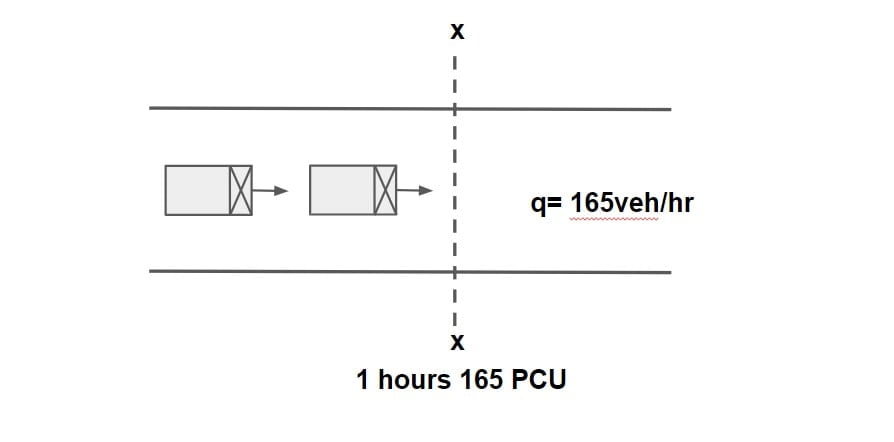
PCU (Passenger Car Unit)

Under mixed traffic conditions, It is difficult to find traffic volume, traffic density etc hence all class of vehicle are converted into a standard vehicle unit which is called PCU.

Class of Vehicle	PCU
Car, Tempo	1
Motar Cycle	0.5
Cycle Rickshaw	1.5
Bus, Truck	3
Horse Drawn Vehicle	4
Small Bullet Car	6
Large Bullet Car	8

\(PCU = \frac{\text{Speed Ratio}}{\text{Length Ratio}}\).

\(PCU = \frac{\frac{V_o}{V_i}}{\frac{L_o}{L_i}}\).

V_o and L_o = speed and length of standard vehicle.

Example: The free speed of a car on a 6 lane road is 120kmph, while that of a truck is 60kmph. The length of the car is 5m, where as the length of the truck is 10m. The PCU of the truck is ……

\(PCU =\frac{\frac{80}{40}}{\frac{5}{40}}=4\)

Measurements of Traffic Volume

Manual Method

In manual counts, trained persons are posted at each lag of an intersection to count and record the number of trucks or buses, cars, etc.

Mechanical Method 

• Radar (Radio Detection & Ranging)
• CCTV Cameras
• Magnetic Detector
• Pressure Sensitive Detectors

Presentation Of Traffic Volume Data  

Traffic Volume Data can be expressed in the following different ways.

1. Annual Average Daily Traffic (AADT)
2. Annual Average Hourly Traffic (AAHT)
3. Annual Average Week Day Traffic (AAWT)
4. Average Daily Traffic (ADT)
5. Trend Chart
6. 30^th Highest Hourly Volume
7. Volume Flow Diagram at Intersection 
8. Variation Chart

i. Annual Average Daily Traffic (AADT)

AADT= \(\frac{\text{Total number of vehicles throughout a years}}{365}\) veh/day.

ii. Annual Average Hourly Traffic (AAHT)

AAHT= \(\frac{\text{Total number of vehicles throughout a years}}{365×24}\) veh/hr.

AAHT= \(\frac{AADT}{24}\) veh/hr.

iii. Annual Average Week Day Traffic (AAWT)

AAWT= \(\frac{\text{Total number of vehicles throughout week days}}{260}\) veh/day.

NOTE: AAWT>AADT, as on weekends traffic volume is considerably reduced.

iv. Average Daily Traffic (ADT)

ADT= \(\frac{\text{Total number of vehicles throughout week}}{7}\) veh/day.

NOTE: ADT>AADT

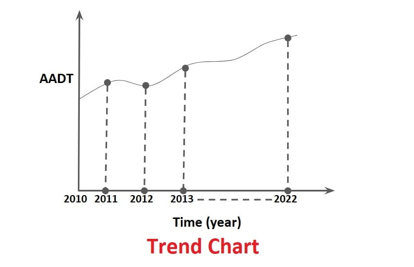
v. Trend Chart

1. Traffic volume data can be represented in form of Trend chart over period of years, which is useful in estimating the rate of growth of traffic that can be used for planning future expansion, design and regulation.
2. If from the trend chart rate of growth of traffic volume is computed to be r%, then future traffic in given by

A=P(1+r)ⁿ

A= future traffic volume

P= present traffic volume

n= no of years.

Note: Average rate of growth of traffic is consider 5-7.5%.

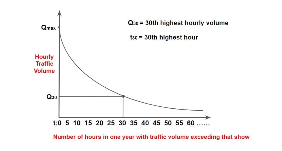
vi. 30^th Highest Hourly Volume

1. It has been observed that 30^th highest hourly volume gives a satisfactory results in terms of performance & it is economical in nature.
2. 30^th highest hourly volume is exceeded only 29 times in a years & all other traffic data will lie lesser than that.
3. IRC consider this traffic volume as Design Hourly Volume.

vii. Volume Flow Diagram at Intersection 

• A volume flow diagram at an intersection either drawn to a certain scale or indicating traffic volume can be used find the details of crossing & turning traffic.
• These data are required for the design of the Intersection.

 

viii. Variation Chart

Variation charts show the hourly, daily, and seasonal variations. It helps in deciding the facilities and regulations needed during peak traffic hours.

NOTE:

Periodic Volume Count 

⇒ To find certain traffic data, such as AADT, ADT etc. it is necessary to count traffic for long duration of time(maybe for years or months).
⇒Counting traffic for a long duration of time, involves cost & effort which is not feasible practically.
⇒Hence to make a reasonable estimate of certain traffic data concept of expansion factor can be used in Periodic Volume Count.
⇒In periodic volume count, expansion factors are used as follows.

1. Hourly Expansion Factor (HEF)

HEF= \(\frac{\text{Total traffic for a day}}{\text{Traffic for particular hour}}\)

2. Daily Expansion Factor (DEF)

DEF= \(\frac{\text{Total traffic for a week}}{\text{Traffic for particular day}}\)

3. Monthly Expansion Factor (MEF)

MEF= \(\frac{AADT}{ADT}\)

Peak Hour Factor (PHF)

It is defined as the ratio between the number of vehicles counted during the peak hour and four times the number of vehicles counted during the highest 15 consecutive minutes. Peak hour factor is a measure of the variation in demand during the peak hour.

\(PHF_{15} =\frac{\text{Hourly traffic volume}}{\frac{60}{15}\times V_{15}(max)}\).

\(PHF_{5} =\frac{\text{Hourly traffic volume}}{\frac{60}{5}\times V_{5}(max)}\).

V₁₅ = maximum number of vehicles during any 15 consecutive minutes

V₅ = maximum number of vehicles during any 5 consecutive minutes.

\(\frac{n}{60}\leq(PHF)_n\leq 1\).

---

B. Traffic Speed Studies

Speed is the rate of travel expressed in kmph or m/s . Over a particular route, the actual speed of vehicle may vary. Speed of a vehicle depends upon several factors such as geometric features, traffic conditions, time, place, driver and environment.

Types of Speed

1. Spot Speed
2. Average Speed
   1. Time Mean Speed
   2. Space Mean Speed
3. Journey Speed
4. Running Speed

a. Spot Speed

It is the instantaneous speed of the vehicle at a particular instant of time or section of road. It is measured by an enoscope, Pressure Contact Tube, and Loop Detector.

b. Average Speed

It is the average speed of traffic calculated based on the spot speed of so many vehicles. It can be considered in two different ways.

1. Time Mean Speed
2. Space Mean Speed

i. Time Mean Speed

The arithmetic mean of spot speed of all vehicle is called Time Mean Speed.

\(V_t= \frac{V_1+V_2….+V_n}{n}\)

ii. Space Mean Speed

It is harmonic mean of spot speed of all vehicle.

\(V_s= \frac{n}{\frac{1}{V_1}+\frac{1}{V_2}….+\frac{1}{V_n}}\)

Note: V_t>V_s

c. Journey Speed

Journey Speed =\(\frac{\text{length of journey}}{\text{time of journey}}\)

d. Running Speed

Running Speed =\(\frac{\text{length of journey}}{\text{Running time}}\)

Running Time = Journey Time – Delay 

Generally, there are two types of speed studies carried out.

1. Spot Speed Study
2. Speed And Delay Study

1. Spot Speed Study

Spot speed studies cannot be used to find density because measurements are done at one point only. Spot speed studies are generally carried out for the following reasons:

• In accident studies
• To calculate the traffic capacity
• Planning of traffic regulations
• Decide the speed trends.

Representation Of Spot Speed Data

• Speed Distribution Table
• Frequency Distribution Curve
• Cumulative Speed of Vehicle

Speed Distribution Table

From the spot speed data of the selected sample, frequency distribution tables are prepared for various speed range and no of vehicle in such range. The arithmetic mean is taken as average speed.

Example

Speed Rang (kmph)	No of Speed / Frequency Observed	% Frequency
0-10	5	1.25
10-20	8	2
20-30	10	2.5
30-40	17	4.25
40-50	30	7.5
50-60	46	11.5
60-70	200	50
70-80	52	13
80-90	32	8
	400

Frequency Distribution Curve

• Curve plotted between average values of each speed group on the x-axis and the frequency of vehicles in that group on y-axis is known as frequency distribution curve of the spot speed.
• A frequency distribution curve of spot speed is plotted with speed of vehicle or avg. value of each speed group of vehicle on the X- axis and the percentages of vehicle in that group on the Y- axis. This graph is called speed distribution curve.

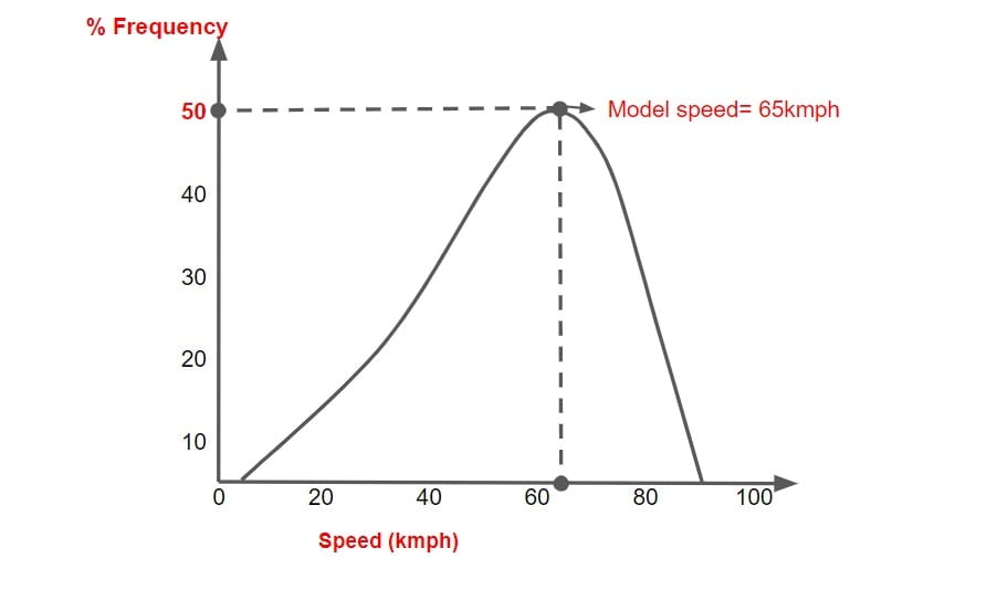
Model Speed

The speed at which greatest number of vehicle travels. It is the peak value of Frequency Distribution Curve.

Cumulative Speed of Vehicle

A graph is plotted between average value of each speed group on x-axis and cumulative percentage of vehicle travelled at or below different speeds on y-axis.

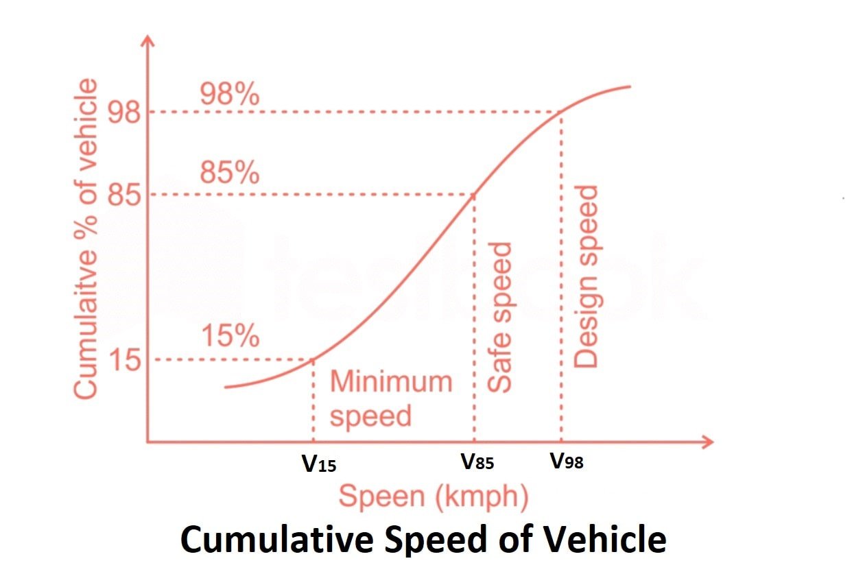
98th percentile speed

It is the speed at or below which 98% of vehicle are moving and only 2% exceeds this limit.

As per IRC this speed is considered as design speed for Geometric design.

85th percentile speed

It is the upper safe movement for vehicle movement.

This is adopted for safe speed limit.

15th Percentile Speed

It is the lower safe limit to avoid congestion.

Minimum speed on Major highway.

50th percentile speed

It is considered as median speed.

2. Speed And Delay Study

We know that spot speed study cannot give the density of traffic. Hence speed & delay studies are carried out over a long distance and hence it is possible to determine density of traffic. This study gives the running speeds, overall speeds, fluctuation in speed and delay between two stations.

There are various methods of carrying out speed and delay study.

• Floating Car Method
• License Plate Method
• Interview Technique
• Elevated Observations

Floating Car Method

• This method is used only for two  lane two road. In this method a test vehicle is driven over a given length of road.
• Speed of text vehicle should be approximately same as speed of traffic.
• A group of four observers sitting in test vehicle records various details.

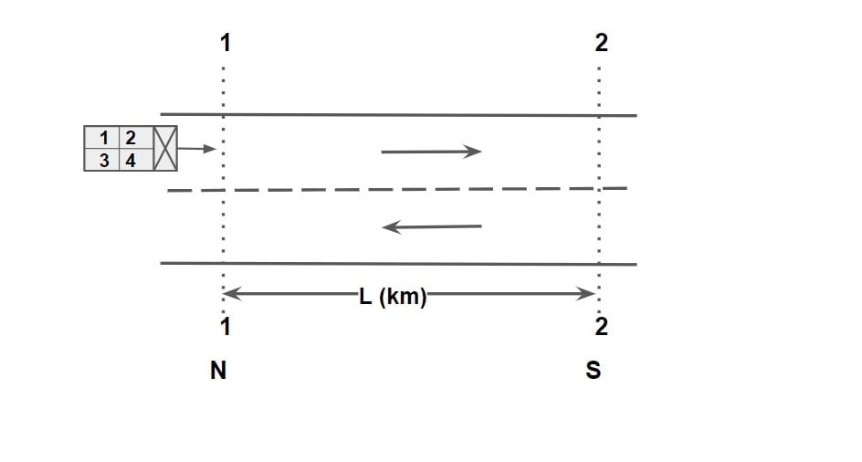Observer 1: 1^st observer will be record total journey time and total cumulative delay time using 2 stop watches.

Observer 2: Location & Reasons for congestion will be noted by 2^nd observer.

Observer 3: Number of vehicle overtaking the test vehicles as well as overtaken by test vehicle will be noted by 3^rd observer.

Observer 4: 4^th observer counts total number of vehicles in opposite direction on adjacent length.

According to this Method

Traffic Flow (q):

\(q=\frac{n_a+n_y}{t_w+t_a}\)

Journey Time of Flow (\(\bar{t} \))

\(\bar{t}=t_w-\frac{n_y}{q}\)

where

t_w= Average journey time when the test vehicle is running with the flow.

t_a= Average journey time when the test vehicle is running against the flow.

n_y= Average no of vehicle overtaking the test vehicle – Average no of vehicle overtaken by the test vehicle.

n_y= overtaking – overtaken. {this can be +ve, -ve or even zero}

n_a= Average no of vehicle counted in the direction of stream when the test vehicle travels in the opposite direction. {n_a is measured by 4th observer of opposite direction of test vehicle}

Derivation Of Floating Car Method

Step.1 When test vehicle stop & all other vehicles is moving.

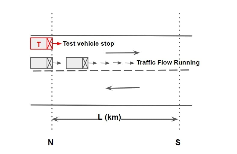
Traffic flow \(q=\frac{n_o}{T} \)

where

T= duration of study

n_o= number of vehicle overtaking the test vehicle

Step.2 When traffic is stop & test vehicle is moving.

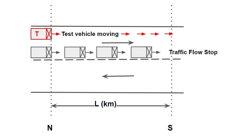
Traffic density \(K=\frac{n_s}{L} \)

n_s= KL= KV_TT

(∴L=V_TT)

n_s= KV_TT

where

n_s= number of vehicle overtaken by test vehicle

Step.3 When test vehicle is moving in the direction of flow & traffic is moving.

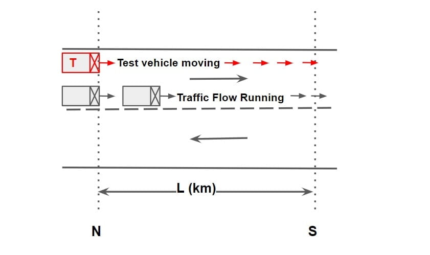
time of journey = t_w

n_y= Average no of vehicle overtaking the test vehicle – Average no of vehicle overtaken by the test vehicle.

n_o= number of vehicle overtaking the test vehicle = qt_w

n_s= number of vehicle overtaken by test vehicle = KL= KV_wt_w

(overtaking – overtaken)= n_y= qt_w – KV_wt_w

n_y= qt_w – KV_wt_w

n_y= qt_w – KL ……….(1)

Step.4 When test vehicle is moving in the opposite direction of flow & traffic is moving.

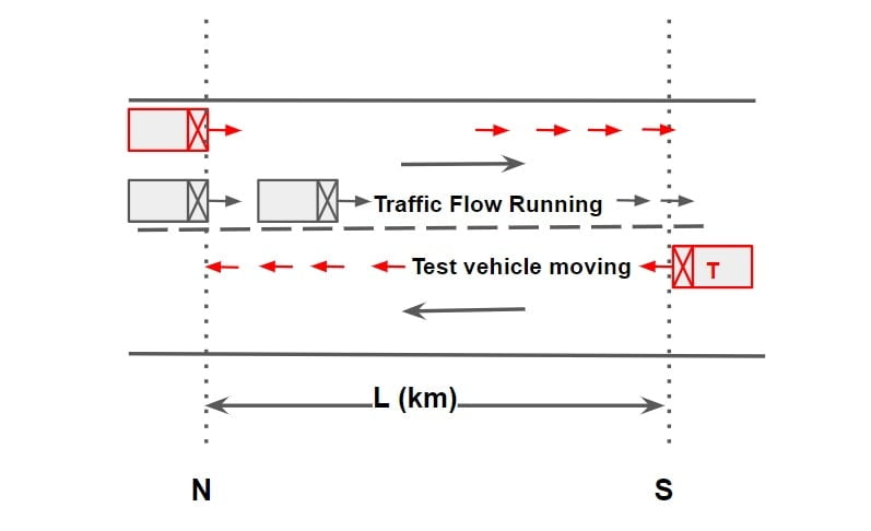time of journey = ta

n_a= Average no of vehicle counted in the direction of stream when the test vehicle travels in the opposite direction

n_a= qt_a + KV_at_a

n_a= qt_a + KL ……….(2)

add equation 1 & 2

ny = qtw – KL  +  na = qta + KL

ny+na = qtw + qta

Traffic Flow (q)

\(q=\frac{n_a+n_y}{t_w+t_a}\)

Journey Time of Flow (\(\bar{t} \))

from equation 1

n_y= qt_w – KL

K= q/v and L=vt

\(n_y=qt_w-\frac{q}{v}\times v\times t\).

\(n_y=qt_w-q\bar{t}\).

Journey time of flow

\(\bar{t}=t_w-\frac{n_y}{q}\)

---

C. Traffic Flow Characteristics & Capacity Study

1. Traffic Capacity Studies
2. Traffic Flow Characteristics Studies

i. Traffic Capacity Studies

Traffic Volume

Number of vehicle crossing the particular section of road is per unit time is called Traffic Volume. It is expressed in veh/day, veh/hr, veh/min.

Traffic Density (K)

Number of vehicle occupied by unit length of the road is called traffic density. It is expressed as vehicle/km, vehicle/metres.

Jam Density (Kj)

Traffic density under jam condition is called jam density. It is the maximum value of traffic density.

Note

• When density reaches to its maximum jam condition developed.
• Jam Condition is the worst condition on road under which congestion is so high, due to which movement of vehicle is not possible, hence speed of vehicle under jam condition is zero.
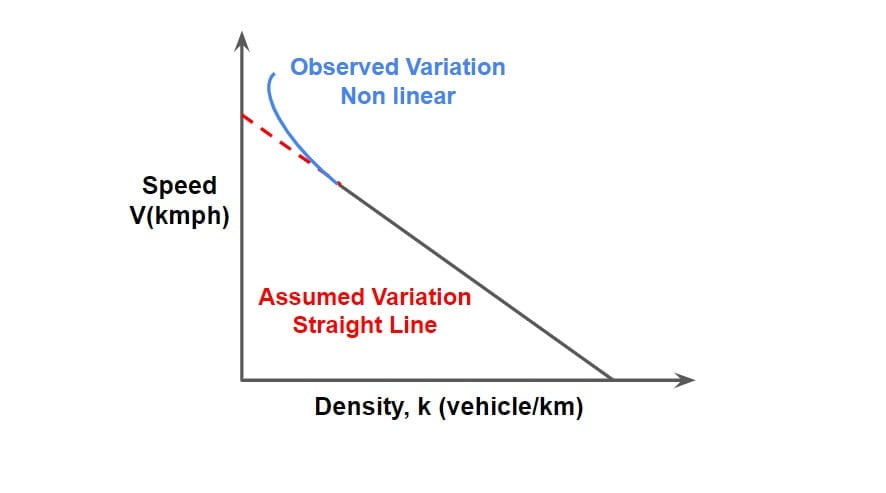
• Traffic Density varies with speed inversely, hence when with increase in speed of a stream vehicle on a roadway, the average density of vehicle decreases. This is because gap of spacing between the vehicle increases

Space Headway (S)

• It is the distance, maintained between two consecutive vehicle travelling in same direction.
• It is the total length occupied by a moving vehicle on road, which includes length of vehicle and the gap between the two vehicle.
• This gap for safety point of view must be equal to SSD to avoid the collision between the two vehicle but this value of gap makes the designing over safe.
• Hence for geometric design this gap is computed by neglecting braking distance & considering reaction time to be 0.7sec instead of 2.5sec.

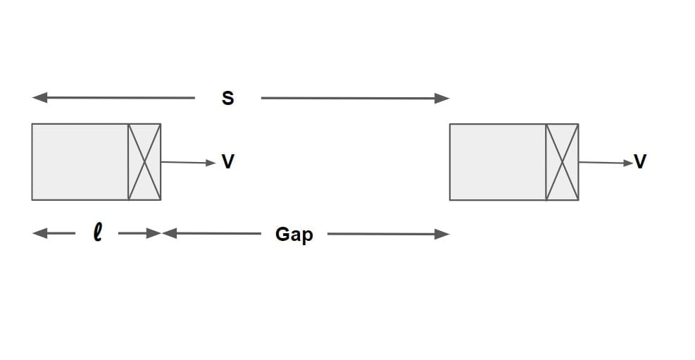
S= Gap + l.

(Gap ⇒ SSD)

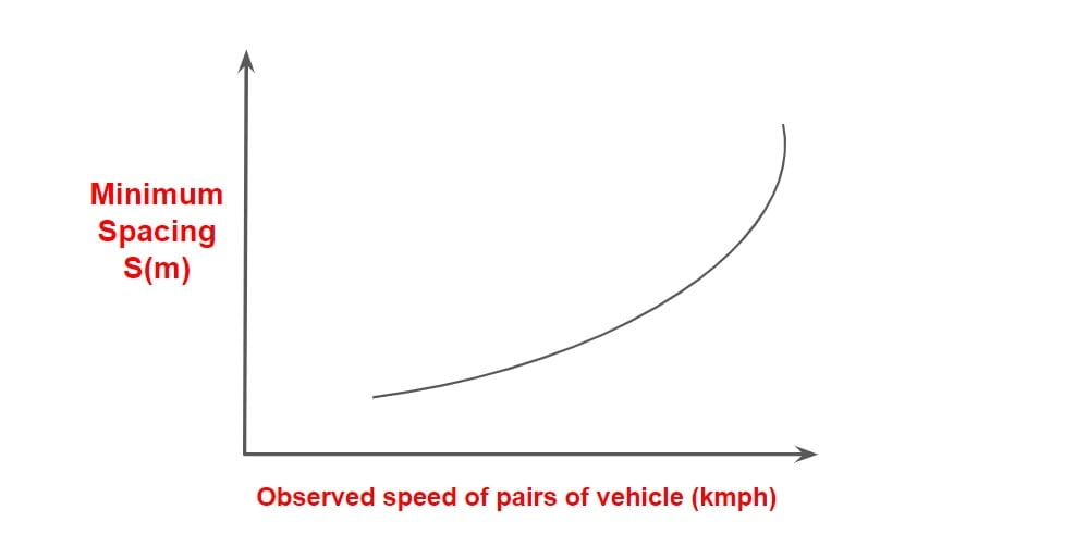
we know that

SSD=\(0.278\times V\times tr\)+ \(\frac{V^{2}}{254(f±s \%)}\)

S = \(0.278\times V\times tr\)+ \(\frac{V^{2}}{254(f±s \%)}\) +l

neglecting braking distance & considering reaction time to be 0.7sec instead of 2.5sec

S = 0.278×t_r×V + l

for geometric design, l= 6m, t= 0.7sec.

S = 0.278×0.7×V + 6

S= 0.2V +6

S= Space Headway in meter V= speed of vehicle in kmph

Hence, Traffic density,

K = \(\frac{\text{1 (km)}}{\text{space headway (m)}}\)

K (veh/km)= \(\frac{1000}{\text{S (m)}}\) 

K  (veh/km)= \(\frac{1000}{0.2V+l}\)

V→km/hr, l→meter, K  → (veh/km)

Note:

Jam density Kj (veh/km)= \(\frac{1000}{l}\)

Under jam condition, V=0 (kmph)

Time Headway (H_T)

It is define as the time gap between passing of two consecutive vehicle travelling in same direction.

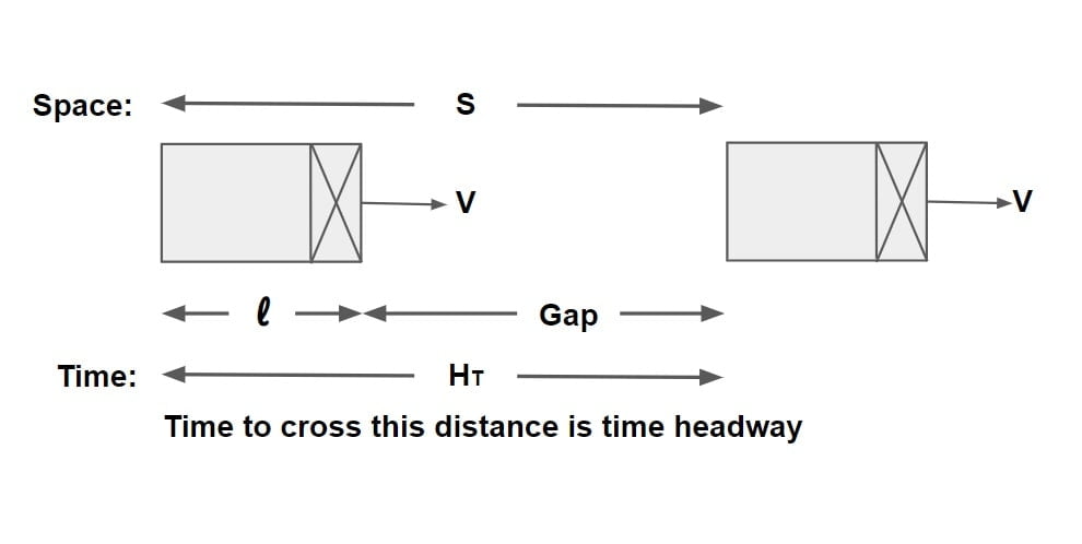Traffic volume,

q= \(\frac{\text{1 hr}}{\text{average time headway}}\)

q (veh/hr)= \(\frac{3600}{{H_T (sec)}}\)

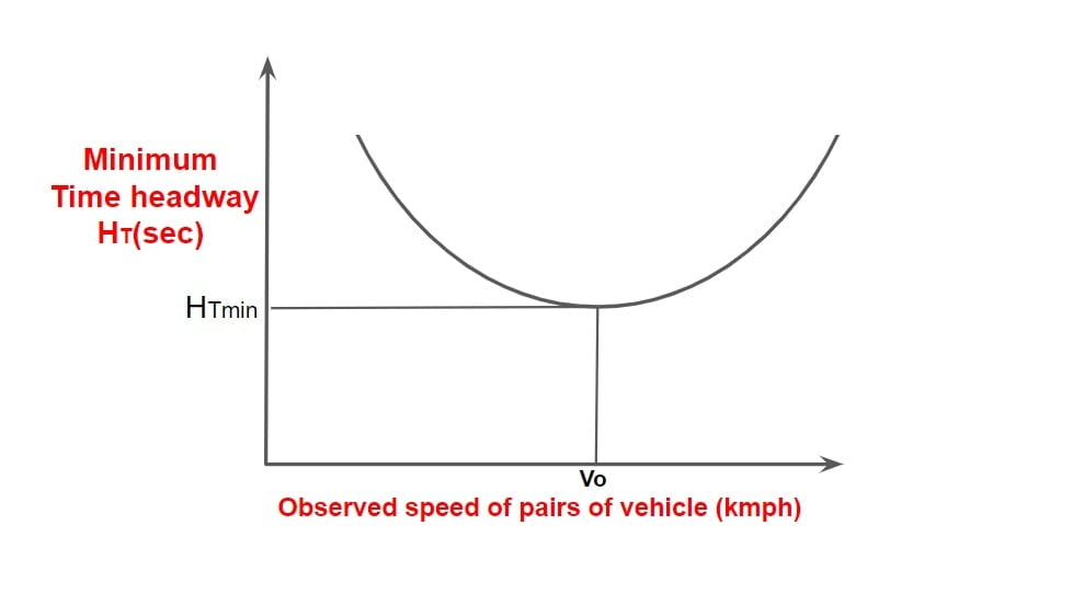
Note.1

• At very low speeds, the time headway is high and number of vehicle crossing a section  on the road is also low. As speed of stream gradually increase, the minimum time headway decreases up to a lowest value at a certain speed.
• The speed at which the value of time headway is lowest represent the optimum speed corresponding max flow or capacity flow.
• If speed of traffic stream is further increased the minimum time headway starts increasing resulting in decrease of traffic flow.

Note.2

Relationship between traffic volume (q), Traffic density (K), and Traffic speed (V).

It is difficult to measure traffic density directly in practical situation, hence the relationship between traffic volume, traffic density and speed is used.

K (veh/km)= \(\frac{\text{q (veh/hr)}}{\text{V (km/hr)}}\)

q= KV

Traffic volume = Traffic Density × Traffic speed

q (veh/hr) = \(\frac{1000}{\text{S (m)}}\) × V (km/hr)

we know that K (veh/km)= \(\frac{1000}{\text{S (m)}}\)

also

q (veh/hr)= \(\frac{\text{3600}}{H_T (sec)}\)

From above two equation of q

\(\frac{3600}{H_T }\)=\(\frac{1000V}{\text{S }}\)

Traffic Capacity

Maximum value of traffic volume, which a road can accommodate is called Traffic Capacity. It is expressed as vehicle per hour per lane. (Traffic Volume ≤ Traffic Capacity). 

Basic Capacity

This Traffic Capacity under most ideal condition is termed as Basic Capacity/Theoretical Capacity.

Note: Two road having the same physical features will have the same basic capacity irrespective of traffic condition, as they are assumed to be ideal.

Practical capacity

It is the maximum number of vehicle that can pass a given point on a roadway during one hour, without traffic density being so great, as to cause unreasonable delay, hazard or restriction to the driver’s freedom to maneuver under the prevailing roadway and traffic conditions.

Note:

• Sometimes practical capacity is also called as design capacity.
• For design purpose we neither use basic capacity or possible capacity as they represents the two extreme cases of roadway and traffic condition. Hence we have another type of capacity called Practical capacity.

Calculation of Theoretical Maximum Capacity 

1. Max Theoretical Capacity from Space Headway
2. Max Theoretical Capacity from Time Headway

Max Theoretical Capacity from Space Headway

q_max = \(\frac{1000 V}{S}\) 

Max Theoretical Capacity of lane,

C = \(\frac{1000 V}{S}\) 

where,

C= Capacity of single lane (vehicle per hour)

V= speed of vehicle (kmph)

S= 0.2V +6 = Space Headway in meter

Max Theoretical Capacity from Time Headway

q_max= \(\frac{3600}{H_T}\)

Max Theoretical Capacity of lane,

C = \(\frac{3600}{H_T}\)

H_T = Minimum time headway in seconds.

ii. Traffic Flow Characteristics Studies 

Traffic flow characteristics are divided under two categories:

1. Macroscopic Characteristics
2. Microscopic Characteristics

Macroscopic Characteristics

It represents how the behavior of one parameter of traffic flow changes with respect to another. There are many types of macroscopic models but we discuss only Green Shield’s Stream Model.

Green Shield’s Stream Model

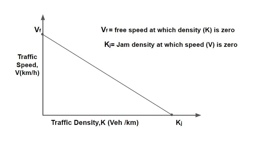
Green shield’s assumed a linear speed- density relationship to derive this model.

The equation for the relationship can be derived as

y= mx +c

V =mK +V_f

m = \(\frac{0-V_f}{Kj-0}\)

m = \(\frac{-V_f}{Kj}\)

V= V_f – \(\frac{V_f}{Kj}\)K

\(V=V_f\left ( 1-\frac{K}{K_j} \right )\)

This equation is referred as “Green Shield’s Stream Model”

now,

q= KV  from previous relationship

q = \(V_f\left ( 1-\frac{K}{K_j} \right )\)K

q = \(V_f\times K-\frac{V_f\times K^{2}}{K_j}\)

using the above relationship, density can be found at which max flow occurs as follows

\(\frac{dq}{dK}=0\)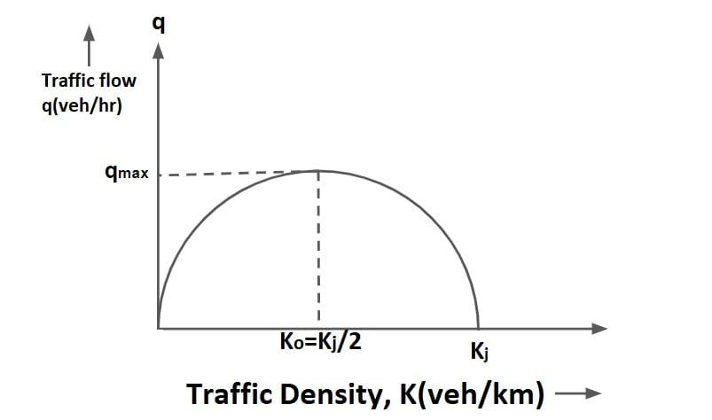

\(V_f-\frac{V_f\times (2K)}{K_j}\)=0

K= K_j/2

Density at which max flow occurs is denoted as optimum density,

K_O= K_j/2

For q_max, put K=K_O=K_j/2 in q

q_max = \(V_f\times \frac{K_j}{2}-V_f\times( \frac{K_j}{2})^{2}\cdot \frac{1}{K_j}\)

q_max = \(\frac{V_f\times K_j}{4}\)

since,

q = \(V_f\times K-\frac{V_f\times K^{2}}{K_j}\)

q= KV ⇒ K=q/V

q = \(V_f\times \frac{q}{V}-V_f\frac{q^{2}}{V^{2}K_j}\)

1 = \(\frac{V_f}{V}-\frac{V_f\times q}{V^{2}\times K_j}\)

\(V^{2}\times K_j=\frac{V_f\times V^{2}\times K_j}{V}-V_f\times q\).

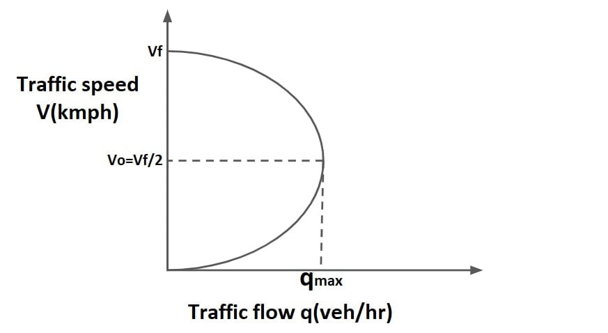
\(q= K_j\times V-\frac{K_j}{V_f}V^{2}\)

to find the speed at which flow is max put K=K_O=K_j/2

V= V_f – \(\frac{V_f}{Kj}\)K

at optimum speed V=V_O, q=q_max

V_O= V_f – \(V_f\frac{K_j}{2}\frac{1}{K_j}\)

V_O= V_f /2

---

Microscopic Characteristics

In Microscopic Characteristics, we discuss about Time headway & Space headway. which already discussed.

Delay & Queue Analysis at Signalized Intersection

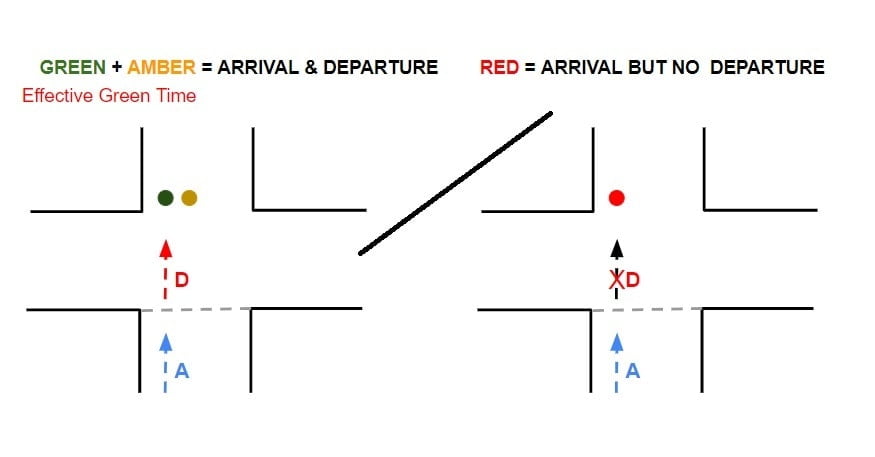
Delay (D)

• It is defined as the time a vehicle is stopped in queue while waiting to pass through signalized Intersection.
• It begins when the vehicle is fully stopped & end when the vehicle begin to accelerate.
• It is mathematically difference departure time & arrival time.
• Average delay is the average for all vehicle during the specified time period.

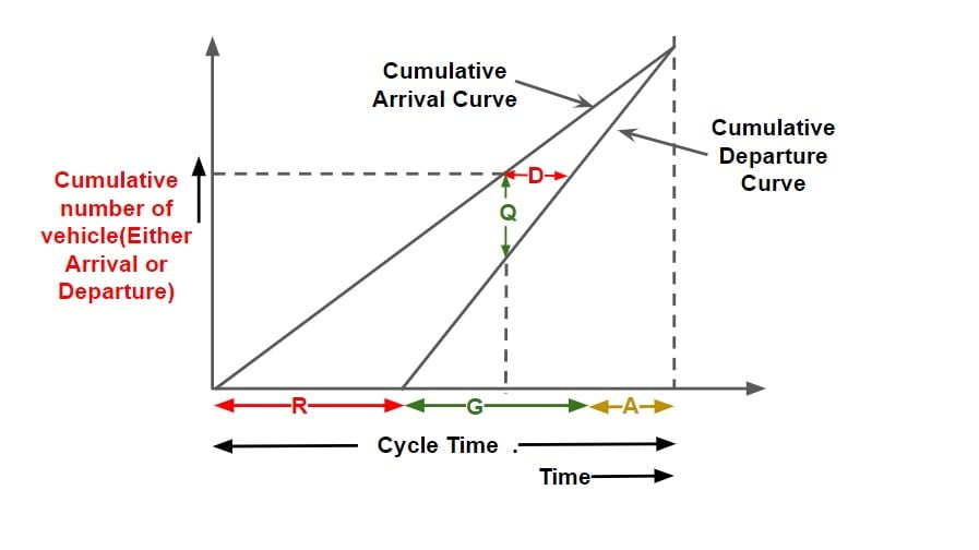
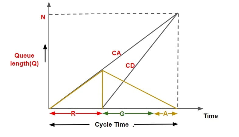
Queue (Q)

• It is the difference of total no of vehicle arrival & total number of vehicle departure at any instant of time.

Note:

Average Delay Per Vehicle =  {Area between cumulative arrival & cumulative departure curve for one cycle time } ÷ {Cumulative number of vehicle arrival per cycle time}

Assumption made in analysis

• Vehicle arrive & departure at uniform rate. (hence cumulative Arrival & cumulative departure curve with time is linear.)
• No pre existing queue is there at intersection.
• Arriving vehicle departs instantaneously when the signal is green.
• The departure of vehicle takes place at it max rate termed as Saturated Flow / Service Rate.
• The departure curve catches up with arrival curve before the next red interval begins.

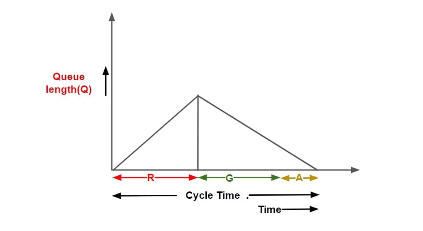
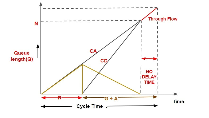
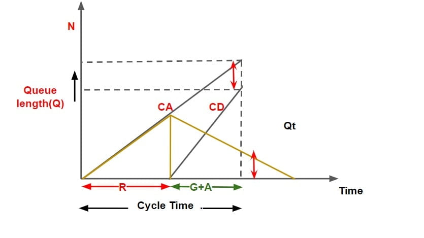
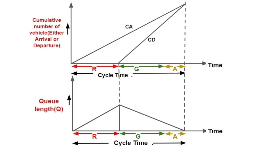Note: Queue length v/s Time Graph can be converted into cumulative arrival & departure v/s time graph.

1. Cumulative departure matches cumulative arrival exactly at the end of one cycle.
2. Cumulative departure matches cumulative arrival before the completion of cycle time.
3. Cumulative departure does not matches cumulative arrival even at the end of one cycle time.

---

---

D. Origin and Destination (O & D) Study

This study is essential in planning new highway facilities or improving existing road systems.

This study is generally carried out to

• To locate intermediate stops of public transport.
• To locate expressways & major routes along the desires line.
• To locate new bridge as per traffic demand.
• To identify potential congestion points.

Method for Origin and Destination data calculation:

1. Road Side Interview Method
2. License Plat Method
3. Tag On Car Method
4. Return Post Card Method
5. Home Interview Method

Representation of Origin and Destination Data

1. O&D Table
2. Desire Lines
3. Pie Chart

O&D Table

• It shows number of trips between different zones.

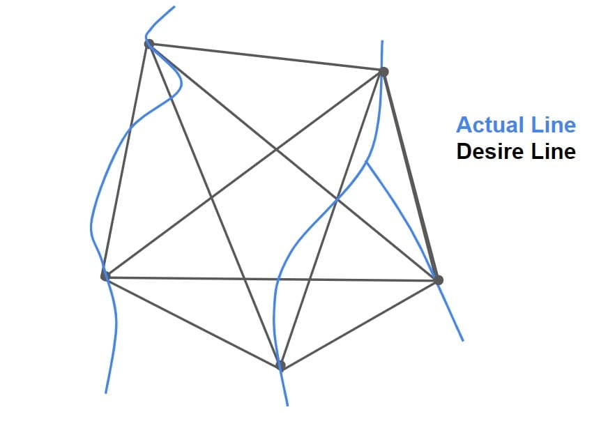
Desire Lines

• O&D data is represented by Desire Line.
• Desire lines are the straight line joining origin to destination.
• The width of desire line is proportional to the number of trips in both directions.
• The desire line density map helps to decide the actual desire of the road user with respect to path to be followed between two points.

Pie Chart

O&D studies data can also be represented in the form ‘Pie Chart’ & ‘Contour Lines’.

---

E. Accident Study

One of the primary goals of traffic engineering is to ensure safe traffic flow. Road accidents cannot be avoided, but they can be significantly minimized with proper traffic engineering.  So, it is essential to analyses every individual accident and maintain zone wise accident records.

The Accident Studies’ goals are as follows:

• To study the cause of accident.
• To support proposed designs.
• To figure out how much money you’ve lost due to accidents.
• To analyze the changes required in existing design.

Accidents are caused by a variety of factors:

• Drivers
• Road Design
• Traffic Conditions
• Weather
• Animals
• Road Conditions
• Vehicle Defects

Types of  Accident

• When a moving car collides with a parked vehicle
• When two vehicles approaching from different directions collide at a intersection
• Head-on collision of two vehicles approaching from opposite directions
• When a moving vehicle collides with a stationary item such as an electric pole, a tree, or a stiff structure.

Mathematical Analysis of Accident Studies

The following assumptions involved in the analysis of accidents are:

• If skid marks are present, then it is assumed that 100% skid occurs.
• If skid marks are not present then free collision is assumed means no brakes are applied.

According to Newton’s law of collision,

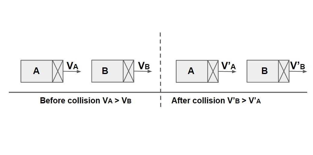
Coefficient of Restitution,

e= \(\frac{\text{Velocity of Separation}}{\text{Velocity of Approach}}\).

e= \(\frac{V_B’-V_A’}{V_B-V_A}\)

Case-1: Elastic Collision

e=1, Velocity of Separation = Velocity of Approach

(V_B‘-V_A‘)= (V_B-V_A)

Case-2: Perfectly Plastic Collision

e=0, Velocity of Separation = 0

(V_B‘-V_A‘)= 0

V_B‘-=VA‘

Both velocity will stick & will more together.

Accident Case Study

When A Moving Vehicle Collides With a Parked Vehicle 

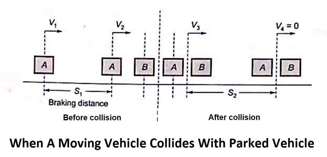Assumption

• Vehicle ‘A’ applies break before collision.
• Braking efficiency is 100%.
• Collision is perfectly plastic.

	Vehicle A	Vehicle B
initial speed	v1	0
speed just before collision	v2	0
speed just after collision	v3	v3
skid before collision	s1	0
skid after collision	s2	s2
mass of vehicle	ma	mb
friction coefficient	f	f

Step-1: Before Collision

ΔKE = work done

\(\frac{1}{2}m_a\cdot v_2^{2}-\frac{1}{2}m_a\cdot v_1^{2}\)=\(-m_a\cdot g\cdot f\cdot s_1\).

\(\frac{v_2^{2}}{2}+gfs_1=\frac{v_1^{2}}{2}\).

\(v_1=\sqrt{v_2^{2}+2gfs_1}\)……(1)

Step-2: At Collision

Momentum just before collision= Momentum just after collision

m_a·v₂+m_b·0= (m_a+m_b)v₃

\(v_2=\frac{m_a+m_b}{m_a}v_3\)……(2)

Step-3: After Collision

ΔKE = work done

\(0-\frac{1}{2}(m_a+m_b)v_3^{2}\)=\(-(m_a+m_b)gfs_2\).

\(v_3=\sqrt{2gfs_2}\)…….(3)

From equation 1, 2 & 3. we will calculate v₁, v₂, v₃.

---

F. Parking Study

One of the primary issues brought on by increased road traffic is parking. Because no vehicle can move on the road for the entire 24 hours of the day, they must stop or park at different locations for different periods of time. As per IRC the standard dimensions of a car is taken as 5× 2.5 metres and that for a truck is 3.75× 7.5 metres.

Parking facilities may be divided into two types.

1. Off-Street Parking
2. On Street/ Kerb Parking

a. Off-Street Parking

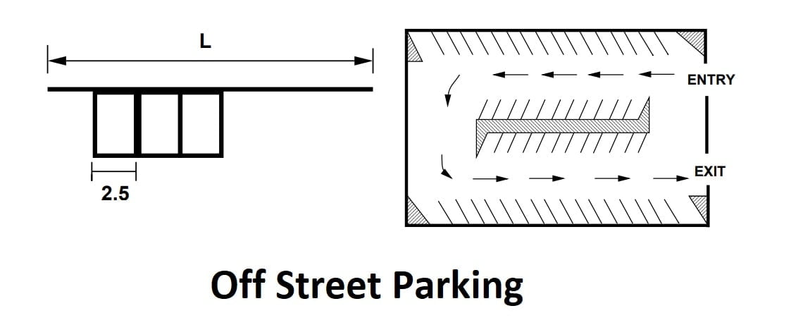
• Off-street parking is given in areas where parking demand is high and kerb parking is not permitted, depending on space availability.
• Vehicles must park away from the kerb in this form of parking.
• The main benefit of this type of parking is that there is no traffic interruption while parking.
• These are further classified into two.
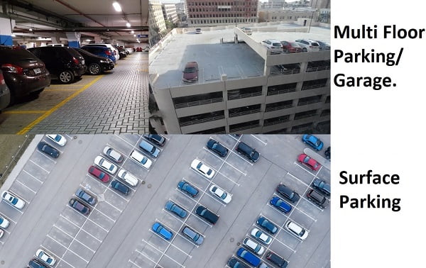
  1. Surface Parking
  2. Multi Floor Parking/ Garage.

 

b. On Street/ Kerb Parking  

• In this type of parking, vehicles are parked along the kerb which may be designed for parking.
• Different patterns of kerb parking are
  1. Parallel Parking
  2. Angle Parking

i. Parallel Parking

• It requires less road width but the number of vehicles that can be parked per unit length of road is least in this case.
• When kerb parking space and street width are limited, it is preferred.
• Parking and un-parking are more complicated and time consuming in this type of parking.

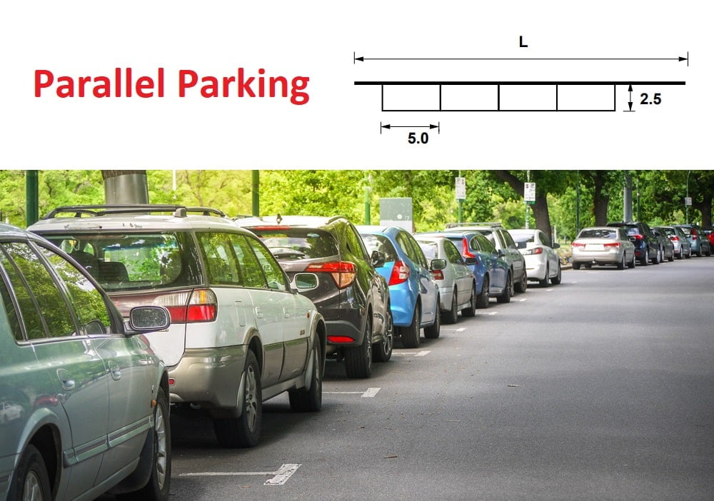
\(N=\frac{L}{5.9}\) (From NPTEL)

\(N=\frac{L}{6.6}\)  (From Coaching Book: Made Easy & IES Master Theory Book)

L= Length of kerb

N= Number of parking spaces.

ii. Angle Parking

• In this case vehicles are being parked at an angle ranging from 30°, 45°, 60°, and 90°.
• it is suitable to be provided where availability of road width is more.
• Angle parking accommodates more vehicle per unit length but maximum vehicles can be parked with an angle of 90°.
• 45° angle parking is considered to be the best.

30° Angle Parking

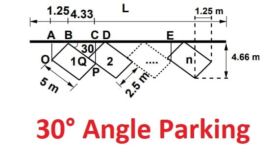
AB = OBsin30◦ = 1.25,
BC = OPcos30◦ = 4.33,
BD = DQcos60◦ = 5,
CD = BD − BC = 5 − 4.33 = 0.67,
AB + BC = 1.25 + 4.33 = 5.58

For N vehicle, L = AC + (N-1)CE =5.58+(N-1)5 =0.58+5N

L = 0.58 + 5N (From NPTEL)

L = 0.85 + 5.1N (From Coaching Book: Made Easy & IES Master Theory Book)

45° Angle Parking

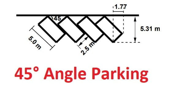
L = 1.77 + 3.54N (From NPTEL)

L = 2 + 3.6N (From Coaching Book: Made Easy & IES Master Theory Book)

60° Angle Parking

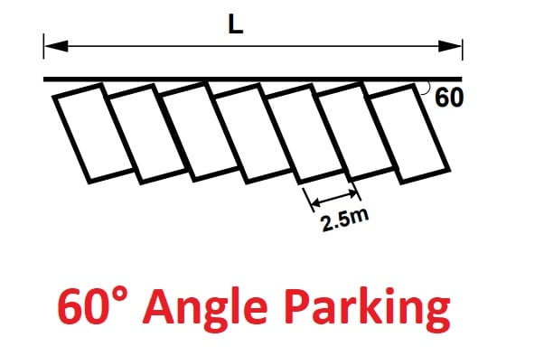L = 2.16+ 2.89N (From NPTEL)

L = 2 + 2.9N (From Coaching Book: Made Easy & IES Master Theory Book)

90° Angle Parking

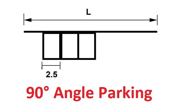L = 2.5N

---

Question: Ratio of width of the car parking area required at kerb for 45° parking relative to 60° parking approximately…..

Solution 

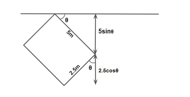
As per IRC, the standard dimension of a car = 5m × 2.5m.

W₄₅ = 5 sin45 + 2.5 cos45 =  5.30

W₆₀ = 5 sin60 + 2.5 cos60 =  5.58

Ratio= \(\frac{W_{45}}{W_{60}} =\frac{5.30}{5.58}\)

Ratio=0.949

---

Parking statistics

Parking Accumulation

• It is defined as the number of vehicles parked at a given instant of time. Normally this is expressed by accumulation curve. Accumulation curve is the graph obtained by plotting the number of bays occupied with respect to time.

Parking Volume

• Parking volume is the total number of vehicles parked at a given duration of time. This does not account for repetition of vehicles. The actual volume of vehicles entered in the area is recorded.

Parking load

Parking load gives the area under the accumulation curve. It can also be obtained by simply multiplying the number of vehicles occupying the parking area at each time interval with the time interval. It is expressed as vehicle hours.

Average Parking Duration

It is the ratio of total vehicle hours to the number of vehicles parked.
Parking Duration = parking load ÷ parking volume

Parking Turnover

It is the ratio of number of vehicles parked in a duration to the number of parking bays available.
parking turnover = parking volume / No of bays available
This can be expressed as number of vehicles per bay per time duration.

Parking Index

Parking index is also called occupancy or efficiency. It is defined as the ratio of number of bays occupied in a time duration to the total space available. It gives an aggregate measure of how effectively the parking space is utilized.

Parking index can be found out as follows
parking index = \(\frac{\text{parking load}}{\text{ parking capacity}}\times 100\)

---

---

  3. Traffic Control Devices & Regulation  

1. Intersection
2. Traffic Signal
3. Traffic Sign
4. Road Marking

A. Intersection  

• Intersection is the area where two or more roads meet or cross.
• At the intersection there are through, turning and crossing traffic movements.
• The movement of traffic are handed depending upon the type of intersection.

There are two type of Intersection.

1. Intersection at Grade
2. Grade Separated Intersection

 i. Intersection at Grade

When all the roads meets at about the same level allowing traffic movements like crossing, weaving, merging & diverging are called “Intersection At Grade”.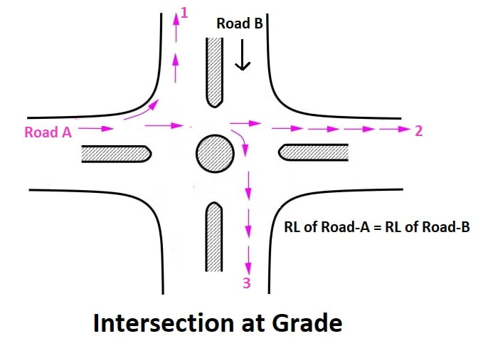

Diverging: It is a traffic operation when the vehicles moving in one direction is separated into different streams according to their destinations.

Merging: Merging is the opposite of diverging. Merging is referred to as the process of joining the traffic coming from different approaches and going to a common destination into a single stream.

Weaving: Weaving is the combined movement of both merging and diverging movements in the same direction.

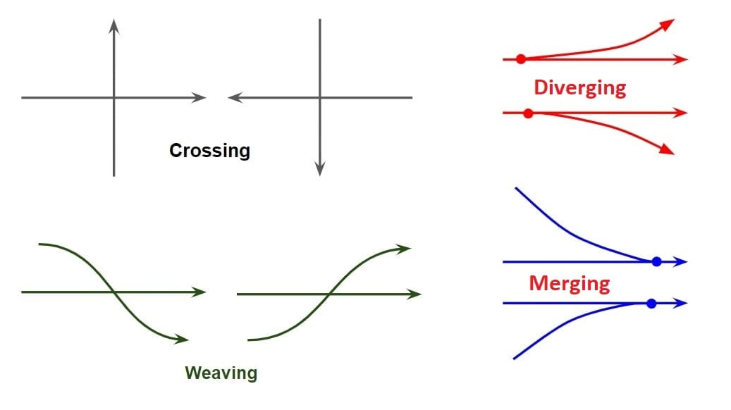
• The point where the possible path of two vehicles intersect is called “Conflict Point”.
• The area containing all possible conflict points is termed as “Conflict Area”.
• If the relative speed & angle of approach of two vehicle is more, it increases the possibility of collision between the vehicle and these conflict point are termed as “Major Conflict Point”. Example- Crossing & Weaving Conflict.
• If the relative speed & angle of approach of two vehicle is less, it decreases the possibility of collision between the vehicle and these conflict point are termed as “Minor Conflict Point”. Example- Merging & Diverging Conflict.
• IRC do not consider Diverging Conflict.

Requirements of Intersection at Grade

The basic requirements of Intersection at Grade are:

• At the intersection, the area of conflict should be as small as possible.
• The relative speed and particularly the angle of approach of vehicle should be small.
• Adequate visibility should be available for vehicles approaching the intersection
• Sudden change of path should be avoided.
• Proper sign should be installed.
• Good lighting at night is desired.

 

 

 

 

 

confits ke examaple and image

 

 

Type of Intersection at Grade

Intersections at Grade are further of following types.

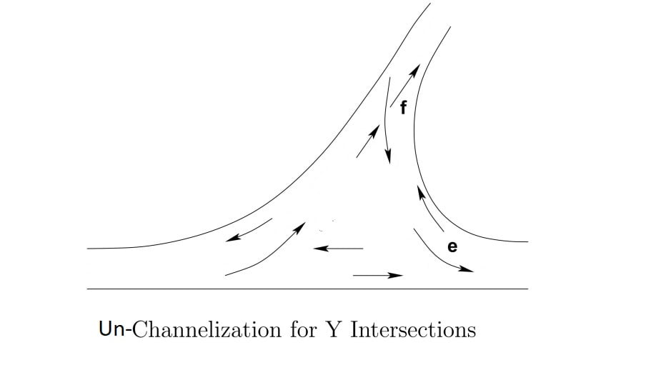
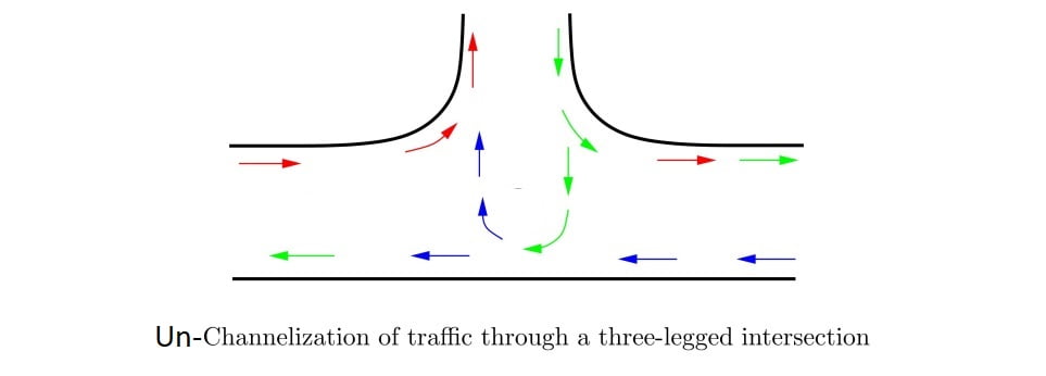
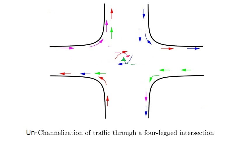
a. Unchannelized Intersections

• In this entire intersection area is paved and there is no restriction to the vehicles to use any part of this intersection area.
• It is very easy to construct but has most complex traffic operation over it resulting in large conflict area.
• It is suitable to be provided for low traffic volume.

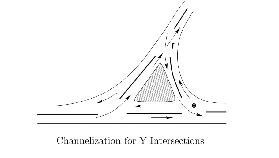
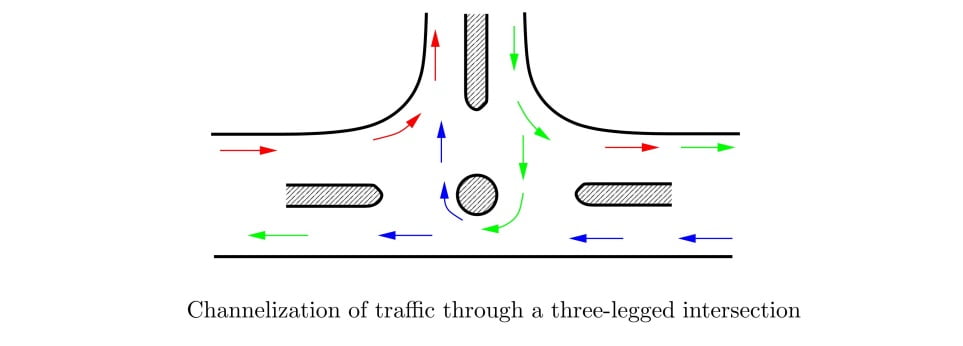
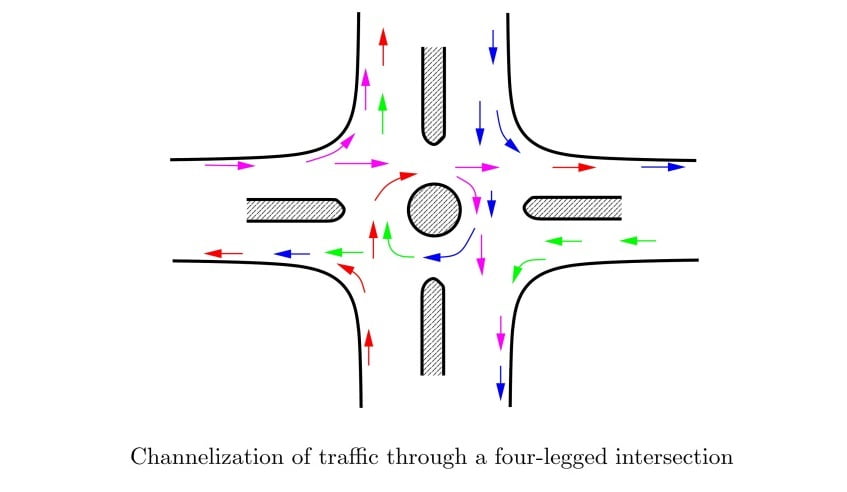
b. Channelized Intersections

• Channelized intersection is achieved by introducing islands into the intersection area, thus reducing the total conflict area available in the unchannelized intersection.
• It is very useful as traffic control devices for intersection at grade and when the direction of the flow is to be changed.
• It is comparatively difficult  to construct.

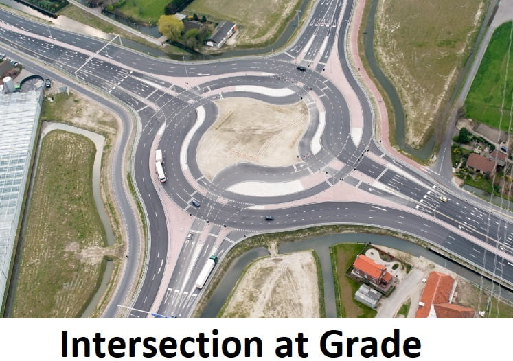
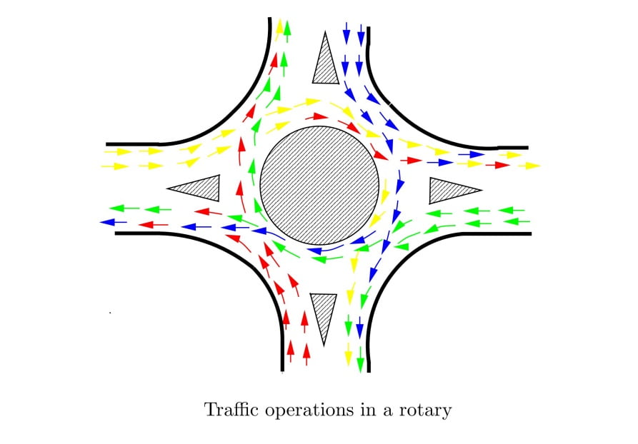
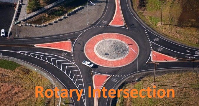
c. Rotary Intersection

It is an enlarged road intersection where all converging vehicles are forced to move round a large central island in clockwise direction before they can weave out of traffic flow into their respective directions.

---

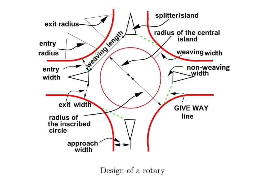
Design Factors For Rotary Intersection

i. Design Speed

Vehicle approaching at grade intersection have to considerable slow down their speed as compared to design speed of that particular road however there is no need for vehicle to stop at rotary.

• For rural area design speed 40kmph.
• For urban area design speed 30kmph.

 

ii. Shape of Rotary Island

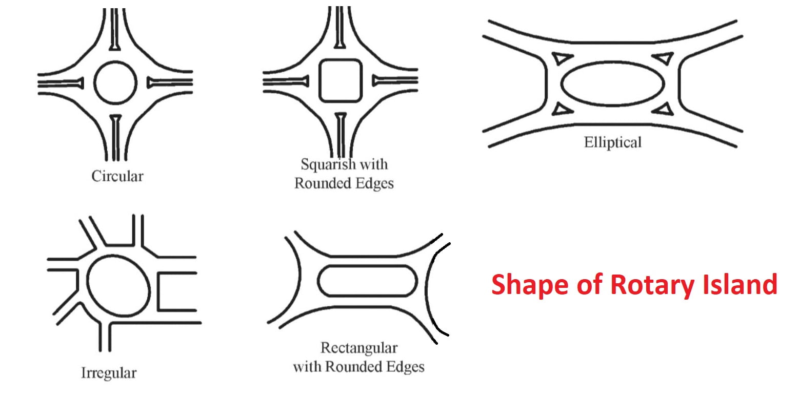
• The shape of central island depends on the number and layout of the Intersecting roads.
• When two equally important roads cross at roughly right angles ie all the four radiating are placed symmetrically, Circular shape is suitable.
• The island may be elongated to accommodate in layout where more than four intersecting road are there termed as elliptical shape
• Tangential shape of rotary is preferred when traffic in one direction is significant compared to traffic in other direction.
• Turbine shape force reduction in speed of vehicles entering the rotary but creates the problem at night of head light glare.

iii. Radius of Curve at Entry 

Radius at entry depends on various factors like design speed, super elevation and coefficient of lateral friction. The entry to rotary is not straight but small curvature is introduced which force the driver to reduce the speed.

e+f = v²/gR = V²/127R

e=0

\(R= \frac{v^{2}}{127f}\)

Hence, Radius of the entry curve is as follows:

Type of Road	Design Speed V(kmph)	Radius (m)
Rural	40	20-35
Urban	30	15-25

iv. Radius of Curve at Exit

Exit radius should be higher than entry radius and radius of rotary island so that vehicle discharge from the rotary at a higher rate.

IRC recommends radius of exit curve to be 1.5→2 time radius of entry curve.

R_exit = (1.5 to 2)× R_entry

v. Radius of Central  Island

IRC recommends radius of central island to be 1.33 time radius of entry curve.

R_C.I = 1.33× R_entry

vi. Width of Carriageway At Exit & Entry

As per IRC width at entry and exit for different lane of approach road are as follows.

For Rural Road

No of lanes	Width of Carriage Way at entry & exit (m),e1
2	6.5
3	7
4	8
6	13

For Urban Road

No of lanes	Width of Carriage Way at entry & exit (m),e1
2	7
3	7.5
4	10
6	15

vii. Width of non-weaving section

The width of non-weaving section of the rotary should be equal to the widest single entry into the rotary and should generally be less than the width of the weaving section(W>e₂).

viii. Width & Length of Weaving Section

The width of non-weaving section (e₂)of the rotary should be equal to the widest single entry into the rotary and should generally be less than the width of the weaving section(W).

The width of weaving section (W) of the rotary should be one traffic lane wider than mean width of the entry & non weaving section, i.e

\(W= \frac{e_1+e_2}{2}+3.5\)

W= e+3.5 m

ix. Length of Weaving Section 

L ≥ 4W

x. Capacity Of Rotary

The practical capacity of rotary is dependent on the min capacity of the individual weaving section and is given by following expression,

Q_p=\([\frac{280W(1+\frac{e}{w})(1-\frac{p}{3})}{(1+\frac{W}{L})}]\)_PCU/hours.

Where,

e= (e₁+e₂)/2 = average width of entry (e₁) & width of non- weaving section (e₂)

L= Length of weaving section

W= width of weaving section

Note

e/W = 0.4 → 1.0

W/L= 0.12 → 0.4

p= Weaving Ratio

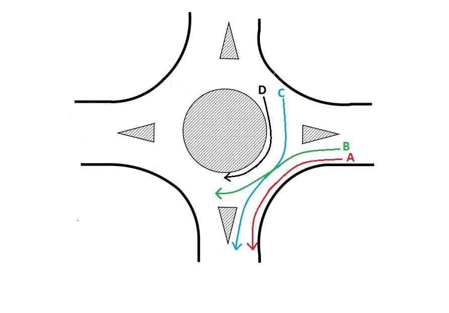
\(p= \frac{b+c}{a+b+c+d}\)

Where,

• a = Left turning traffic moving along left extreme lane
• b = Crossing/Weaving traffic turning towards right while entering to the rotary
• c = Crossing/Weaving traffic turning towards left while leaving rotary
• d = Right turning traffic moving along right extreme lane

Conditions to apply the above formula of capacity of rotary are:

1. 6 m ≤ width of weaving section (w) ≤ 18m
2. e/W = (0.4 – 1)
3. W/L = 0.12 – 0.4
4. p = (0.4 – 1)
5. L = 18 – 90m

---

ii. Grade Separated Intersection

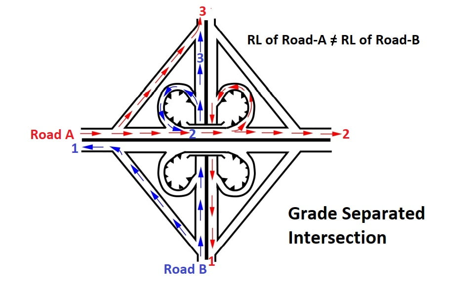
• Grade separation structures that permit the cross flow of traffic at different levels without interruptions.
• Transfer of route at grade separation or turning facilities are provided by “INTERCHANGE” which may be of following types.

Interchange can also be classified based on shape as follows

1. Diamond interchange
2. Trumpet interchange
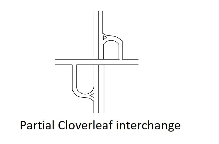
3. Partial Cloverleaf interchange
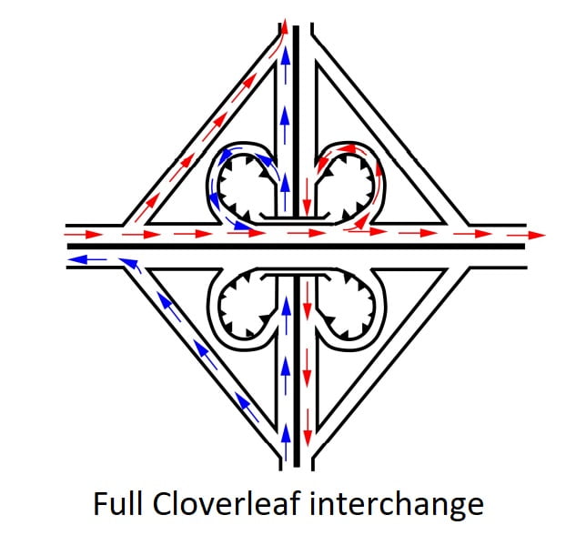
4. Full Cloverleaf interchange

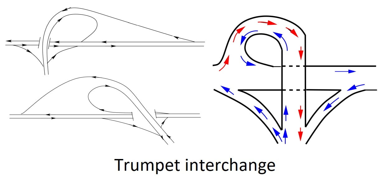
A. Trumpet interchange

Trumpet interchange is a popular form of three leg interchange. If one of the legs of the interchange meets a highway at some angle but does not cross it, then the interchange is called trumpet interchange.

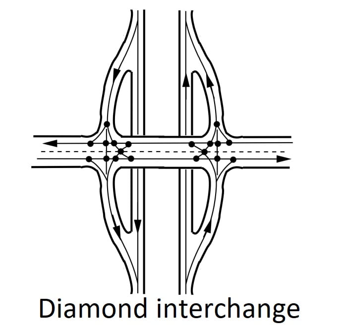
B. Diamond interchange

Diamond interchange is a popular form of four-leg interchange found in the urban locations where major and minor roads crosses. The important feature of this interchange is that it can be designed even if the major road is relatively narrow.

C. Full Cloverleaf interchange

It is also a four leg interchange and is used when two highways of high volume and speed intersect each other with considerable turning movements. The main advantage of cloverleaf intersection is that it provides complete separation of traffic. In addition, high speed at intersections can be achieved. However, the disadvantage is that large area of land is required. Therefore, cloverleaf interchanges are provided mainly in rural areas.

D. Partial Cloverleaf interchange

This is another variation of the cloverleaf configuration. Partial clover leaf or parclo is a modification that combines some elements of a diamond interchange with one or more loops of a cloverleaf to eliminate only the more critical turning conflicts. This is the most popular freeway -to- arterial interchange. Parclo is usually employed when crossing roads on the secondary road will not produce objectionable amounts of hazard and delay. It provides more acceleration and deceleration space on the freeway.

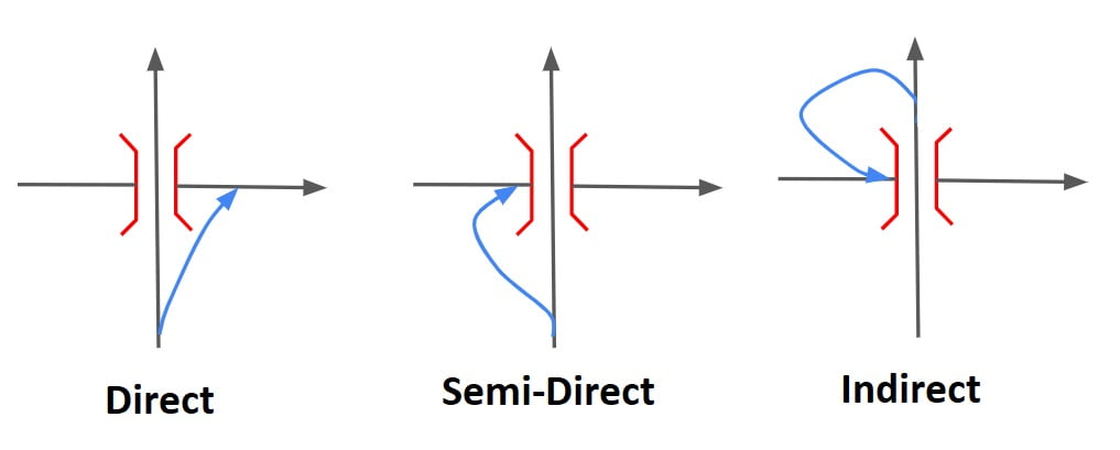
Advantages of Grade Separation

• There is increased safety for turning traffic and by indirect interchange ramp even right turn movement is quite easy and safe.
• There is overall increase in comfort and convenience to the road users.
• Stage constructions of additional ramps are possible after the grade separation structure between main roads are constructed.

Disadvantages of Grade Separation

• It is very costly to provide complete grade separation and interchange facilities.
• Construction of grade separation is difficult and undesirable in the area where there is limited right of way.
• In flat or plain terrain, grade separation may introduce undesirable sags in the vertical alignment.

---

---

B. Traffic Signals

Traffic signals are control devices that could alternately direct the traffic to stop and proceed at intersections using red and green traffic light signals.

The main requirement of traffic signals are

• It should draw the attention of road user.
• It should provide meaning & time to respond.
• It should have minimum waste of time.

  Type of Traffic Signals

The signals are classified into the following types:

1. Traffic Control Signals
   1. Fixed-time Signal
   2. Manually Operated Signal
   3. Traffic Actuated (automatic) Signal
2. Pedestrian Signal
3. Special traffic Signal

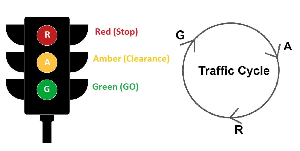
a. Traffic Control Signals

Traffic Control Signals have three colored light glows facing each direction of traffic flow. The Red light is meant for “Stop“, Green light indicates “GO” and the Amber light allows the clearance time for the vehicles which enter the intersection area by the end of green time.

Traffic control signals are of three types:

i. Fixed-time Signal

In Fixed Time Signal the timing of each phase of the cycle is predetermined base on the traffic studies. The main drawback of this is that some times the traffic flow on one road may be almost nil and traffic on cross road may be quite heavy but signal operates with fixed timings.

ii. Traffic Actuated (automatic) Signal

Traffic actuated signals are those in which the timings of phase and cycle are changed according to traffic demand.

• Semi-actuated Signal is a signal whose timing (cycle length, green time, etc.) is affected when vehicles are detected (by video, pavement embedded inductance loop detectors, etc.) on some, but not all, approaches. This mode of operation is usually found where a low-volume road intersects a high-volume road. In such cases, green time is allocated to the major street until vehicles are detected on the minor street: the the green indication is briefly allocated to the minor street and then returned to the major street.
• Fully Actuated Signal is a signal whose timing (cycle length, green time, etc.) is completely influenced by the traffic volumes, when detected, on all of the approaches. Fully actuated signals are most commonly used at intersections of two major streets.

iii. Manually Operated Signal

These signals are operated manually and not commonly used. In these types of signals, the traffic police watches the traffic demand from a suitable point during the peak hours at the intersection and varies the timings of these phases and cycle accordingly.

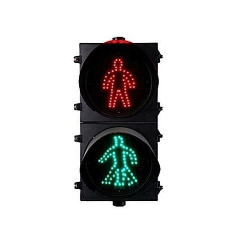
b. Pedestrian Signal

It is used to give the right of way to pedestrians to cross a road when the vehicular traffic shall be stopped by stop signal.

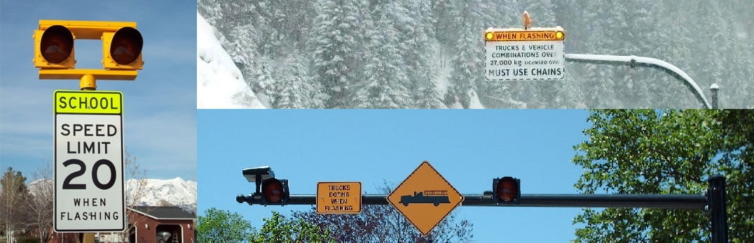
c. Special Traffic Signal

Special traffic signal such as “FLASHING BEACONS” are meant to Warn the traffic. When signal is flashing red then the vehicles shall stop before entering the nearest crosswalk at an intersection.

While flashing yellow signals are caution signals meant to signify that drivers may proceed with caution.

---

  Type of Co-ordination of Traffic Signal System

There are four general types of co-ordination of Traffic signals system

1. Simultaneous System
2. Alternate System
3. Simple Progressive System,
4. Flexible Progressive System

Simultaneous System

• In this system all the signals along a given road always show the same indication (green, red etc.) at the same time.
• As the division of cycle in also the same at all intersections, this system does not work satisfactorily

Alternate System

• It shows opposite indications in a route at the same time.
• This system generally in considered to be more satisfactory than the simultaneous system

Simple Progressive System

• Signals used: fixed time signals
• A time schedule is made to permit, as nearly as possible a continuous operation of groups of vehicles along the main road at a reasonable speed.
• Disadvantage: Cannot co-ordinate a large series of signals. As problem may be created for other routes.

Flexible Progressive System

• In this system it is possible to automatically vary the length of cycle, cycle division and the time schedule at each signalized intersection with the help of a computer.
• This is the most efficient system of all the four types described above.

---

  Important Terminology of Traffic Signals

1. Cycle

A signal cycle is one complete rotation through all the indications provided. (Red, Green, Amber)

2. Cycle Length (C)

It is the time in seconds that it takes a signal to complete one full cycle of indication ie. the time interval between the starting of green for one approach till next time the green starts.

3. Interval

It indicates the change from one stage to another. There are two types of interval:

1. Change Interval: It is also called yellow time and it indicates the interval between green and red Signal.
2. Clearance Interval: It is also known as all red time and is included after each yellow interval indicating a period during which all signal phases shows red and it is used for clearing of vehicles at the intersections.

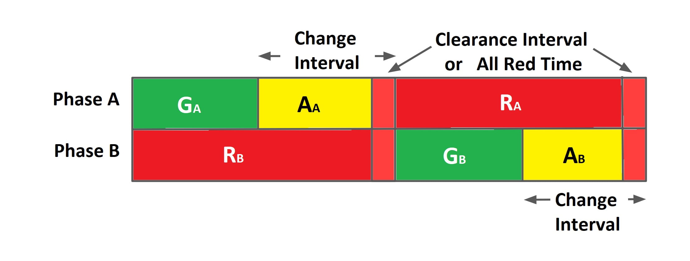
C = G_A +A_A + R_A 

or C = G_B +A_B + R_B

G_A +A_A = R_B

G_B +A_B = R_A

Hence C = G_A +A_A + G_B +A_B

or  C = R_A +R_B

Note: Clearance interval is provided after yellow interval & is optional, hence if the intersection is small then there is no need of clearance interval.

4. Green Time

It is provided to allow traffic flow through the intersection. It is designed on the basic of traffic volume of given road. It is the actual time duration the green signals is turned on.

5. Red Time

It is provided to stop the traffic flow on the intersection. It is designed on the basic of traffic volume of cross road. It is the actual time duration the red signals is turned on.

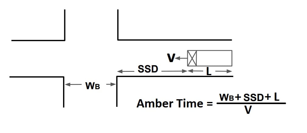
6. Amber Time

It is clearance time provided after the green time, just for clearance of traffic so that traffic on cross road can be started.

7. Phase

8. Lost Time (t_L)

• It is the time during the phase which is not utilized effectively for vehicle movement.
• Total lost time is combination of
  1. Startup Lost Time (t_SL)
  2. Clearance Lost Time (t_SL)

Startup Lost Time (t_SL)

• It is the lost at startup at green time.
• At the start of green time the driver standing very near to the queue usually take sometime to react & some accelerate the vehicle. This lost time is know as Startup Lost Time (t_SL).

Clearance Lost Time (t_CL)

• There is a psychological tendency of driver not to use later portion of the amber, which is called clearance lost time.

---

9. Effective Green Time (g_i)

Effective green time is the actual time available for vehicle to cross the intersection.

g_i= Gi + A_i – t_L

where,

Gi = Actual green time

A_i= Amber time

t_L =Lost time

10. Lane Capacity

If C = cycle length (in second), then number  of cycles in an hour is = 3600/C

Total effective green time in an hour = (3600/C) ×g_i

If h = time headway is seconds for the vehicles crossing the intersection, then total no. of vehicles crossing the intersection in one hour = {(3600/C) ×g_i} ÷ h

=\(\frac{3600}{h}\frac{g_i}{C}\)

capacity of a lane in veh/hr =\(\frac{3600}{h}\frac{g_i}{C}\)

\(\frac{3600}{h}\) = Saturation Capacity, \(\frac{g_i}{C}\)=green ratio.

---

  Method of Signal Designing

There are various method of signal designing:

1. Trial Cycle Method
2. Approximate Method
3. Webster Method
4. IRC Method

For Gate and IES point of view only Webster Method in syllabus.

Webster Method

In this method the optimum cycle length (C_O) calculated on the basis of least total delay to the vehicles at the signalized intersection.

Optimum cycle time, C_O= \(\frac{1.5L+5}{1-Y}\) seconds

where,

L = Total time lost = nt_L + R

n = Number of phase

t_L= Lost time = Startup Lost Time (t_SL) + Clearance Lost Time (t_SL)

R = All red time

For the average signal cycle, the lost time (t_L) is taken to be 2 seconds.

Total time lost,

L = 2n+R  (∴t_L=2)

and,

Y= y_A+y_B

\(y_A=\frac{q_A}{S_A}\).

\(y_B=\frac{q_B}{S_B}\)

where,

q_A or q_B= Normal flow in road A/B in veh/hr/lane

S_A or S_B = Saturation flow in road A/B in veh/hr/lane

Green time for road A is given by,

G_A = \(\frac{y_A}{Y}\) (C_O-L) sec

and

Green time for road B is given by,

G_B = \(\frac{y_B}{Y}\) (C_O-L) sec

---

Example.1

Design two phase traffic signal by webster’s method using the following data:

Road	Average Normal Flow (veh/hr)	Saturation Flow (veh/hr)
A	400	1250
B	250	1000

The all red time required for pedestrian crossing is 12 sec. Design two phase traffic signal by webster’s method.

Solution

C_O= \(\frac{1.5L+5}{1-Y}\)

L = nt_L + R = 2n +R = 2×2+12

L = 16sec

\(y_A=\frac{q_A}{S_A}\).

\(y_A=\frac{400}{1250}\)

y_A = 0.32

\(y_B=\frac{q_B}{S_B}\).

\(y_B=\frac{250}{1000}\)

y_B = 0.25

Y= y_A +  y_B =0.32 + 0.25 = 0.57

C_O= \(\frac{1.5\times 16+5}{1-0.57}\)

C_O = 67.5sec

G_A = \(\frac{y_A}{Y}\) (C_O-L) sec

G_A = \(\frac{0.32}{0.57}\) (67.5-16) =28.9sec

G_A ≈ 29 sec

G_B = \(\frac{y_B}{Y}\) (C_O-L) sec

G_B = \(\frac{0.25}{0.57}\) (67.5-16) = 22.58sec

G_B = 22.6sec

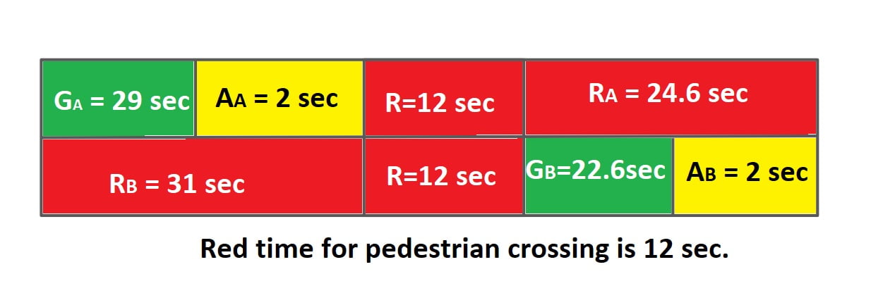
Providing amber time of 2 sec for each phase for clearance.

For Phase A

G_A = 29 sec

A_A = 2 sec

R_A = G_B +A_B = 22.6 + 2 = 24.6 sec

Red time for pedestrian crossing is 12 sec.

For Phase B

G_B = 22.6 sec

A_B = 2 sec

R_B = G_A +A_A = 29 + 2 = 31 sec

Red time for pedestrian crossing is 12 sec.

---

Example.2

A fixed time two phase traffic signal is to be designed for an urban intersection using Webster’s approach. The intersection is having N-S and E-W roads, where any straight ahead traffic is permitted. The design hourly traffic flow from various arms & the corresponding saturation flow are given as follow compute optimum cycle length by assuming all red period per phase & time lost per phase due to starting delay as 3 second and 2 second respectively.

Arms of Intersection	Design hour Traffic Flow (PCU/hr)	Saturation Traffic Flow (PCU/hr)
North	1000	3000
South	600	2400
East	950	3600
West	800	2000

Solution

C_O= \(\frac{1.5L+5}{1-Y}\)

L = nt_L + R = 2×2 + 3×2 =10 sec

y₁ = (1000/3000=0.33 or 600/2400= 0.25)max

y₁ = 0.33

y₂ = (950/3600=0.33 or 800/2000= 0.4)max

y₂ = 0.4

Y= y₁+y₂ =0.733

C_O= \(\frac{1.5\times 10+5}{1-0.733}\)

C_O = 75sec

---

C.  Traffic Sign

A traffic sign is a device that is installed on a fixed or portable support and conveys a specific message using words or symbols. Traffic signs should be set in such a way that they are easily seen and recognized by road users.

Classification of Signs

Traffic sign are divided into 3 categories.

1. Regulatory/Mandatory Signs
2. Warning Sings
3. Informatory Sign

There are three basic types of traffic sign: signs that give orders, signs that warn and signs that give information. Each type has a different shape. Circles give orders, Triangles warn and Rectangles inform.

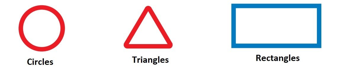
A further guide to the function of a sign is its color. Blue circles give a mandatory instruction, such as “Compulsory Turn Left” etc. Blue rectangles are used for information signs. All triangular signs are red.

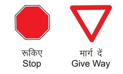
There are a few exceptions to the shape and color rules, to give certain signs greater prominence. Examples are the “STOP” and “GIVE WAY”.

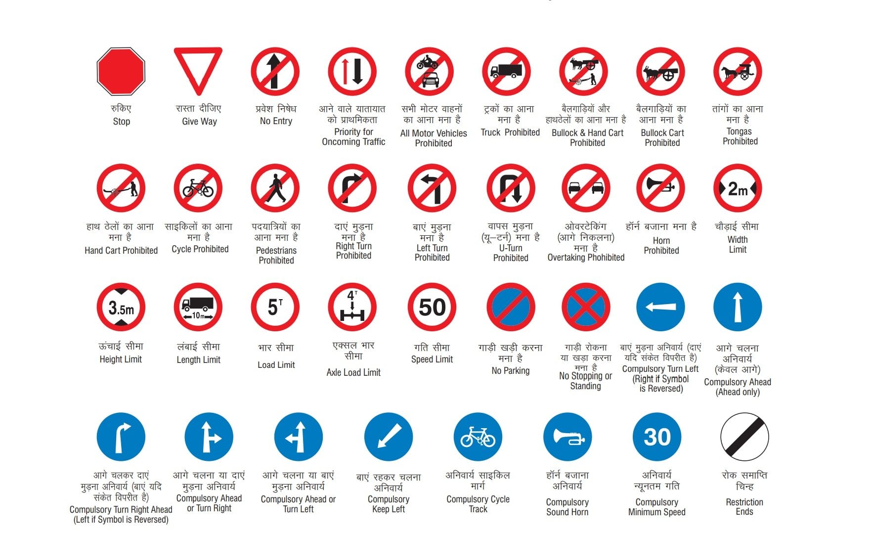
i. Regulatory / Mandatory Signs

Regulatory or Mandatory signs are used to educate road users of specific laws and regulations in order to ensure traffic safety and flow. Violating these signs is a criminal offence.

Shape → Circular (Few exceptions to the shape and colour rules. Examples are the “STOP” and “GIVE WAY”.)

The Regulatory signs are classified under the following sub-heads:

1. Stop and Give-way signs
2. Prohibitory signs
3. Speed Limit and Vehicle Control Signs
4. No Parking and NO Stopping signs
5. Compulsory Direction Control and Other Signs
6. Restriction Ends sign

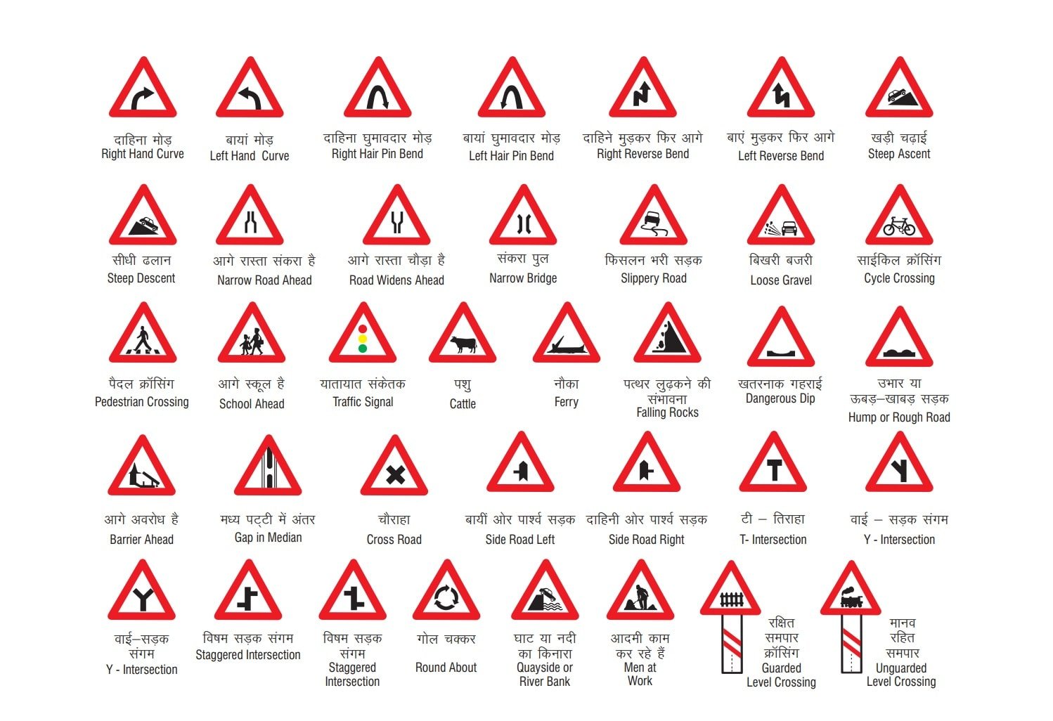
ii. Warning/ Cautionary Sings

These signs are used to advise road users of upcoming road conditions at a suitable distance in advance. Warning signs are also known as cautionary signs. The warning signs are shaped like an equilateral triangle with an upward pointing apex.

Shape → Triangle

The symbols are black and have a white background with a red border.

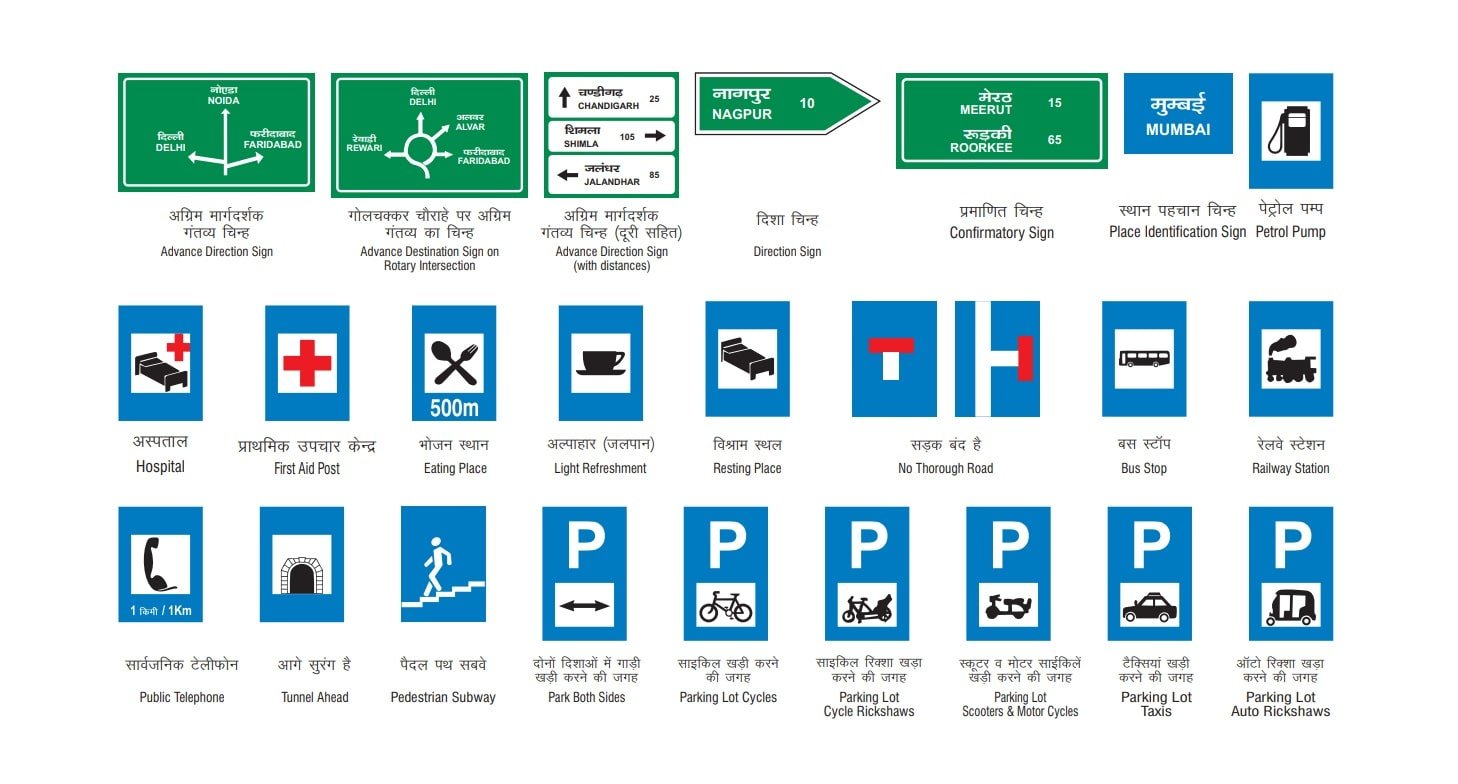
iii. Informatory Sign

Informatory signs are provided to guide the road users about the routes, destination, direction, roadside facilities which make travel easier, safe and pleasant.

Shape → Rectangular

The Informatory Sign are classified under the following sub-heads:

1. Direction and Place Identification signs
2. Facility Information signs
3. Other Useful Information signs
4. Parking sings
5. Food Gauge

IRC recommendations for the design of traffic signs:

1. On high-speed routes, put up large signage.
2. Use no more than three words.
3. Reflectize of illuminate the signs to be read at night.
4. The size of the letters on the sign and the speed of the cars will determine where the signs are placed.
5. Two signs for different purposes should not be placed on the same sign post and should, if possible, be separated by at least 30 meters.
6. Location of the signs with respect to the carriageway.

---

D. Road Marking

Road marking or traffic markings are made of lines, patterns, words, symbols or reflectors on the pavement, kerb, sides of islands or on the fixed objects within or near the roadway. A road marking is a safety device used on a road. Traffic markings may be called special signs intended to control, warn, guide or regulate the traffic. The markings are made using paints in contrast with color and brightness of the pavement or other back ground. Light reflecting paints are also commonly used for traffic marking. In order to ensure that the markings are seen by the road users, the longitudinal lines should be at least 10 cm thick and the transverse lines should be made in such a way that they are visible at sufficient distance in advance to give road users adequate time to respond.

Functions of Road Markings

The main functions of the road markings are to guide the safe and smooth flow of traffic in the
following ways:

• Segregation of traffic
• Stop and Go
• Give way instruction
• Overtaking or not
• Two lanes to one lane/ lane traffic
• Inter-vehicle distance
• Parking zone or no parking
• Speed indication
• Direction
• One way
• Pedestrian crossing
• Type of vehicles allowed

Types of Road Marking

The various types of markings may be classified as,

1. Pavement Marking
2. Kerb Marking
3. Object Marking
4. Reflector Unit Marking

a. Pavement Marking

Pavement markings are made generally with white color & yellow color marking are used to indicate parking restriction. Some of the common types of pavement marking are given below:

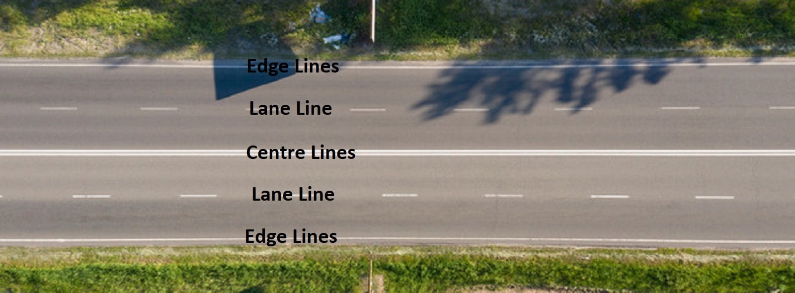
Centre Lines

• These are meant to separate the opposing streams of traffic on undivided two-way roads.

Lane Line

• Lines are drawn to designate traffic lanes. These are used to guide the traffic and to properly utilize the carriageway.

Edge Lines

• Indicate carriageway edge of rural road which have no kerb stones along edge.

No Passing Zone Marking

• These are marked to indicate that overtaking is not permitted.

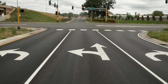
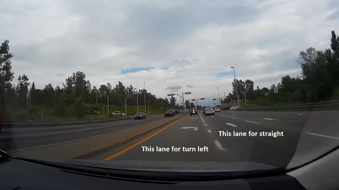
Turn Markings

• These are useful near intersection to designate proper lateral placement of vehicles before turning to the different directions.

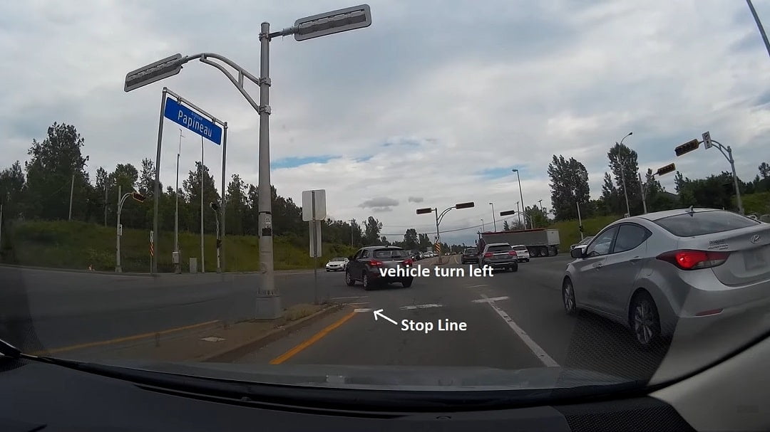
Stop Line

• These are meant for vehicles to stop near the pedestrian crossing, signalized intersection etc. where the vehicles have to stop and proceed.

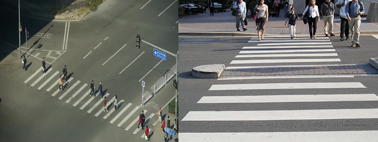
Crosswalk Lines

The particular places where pedestrian are to cross the pavement are properly marked by the pavement markings. The width of pedestrian crossing may be between 2.0 and 4.0 m depending on local requirements.

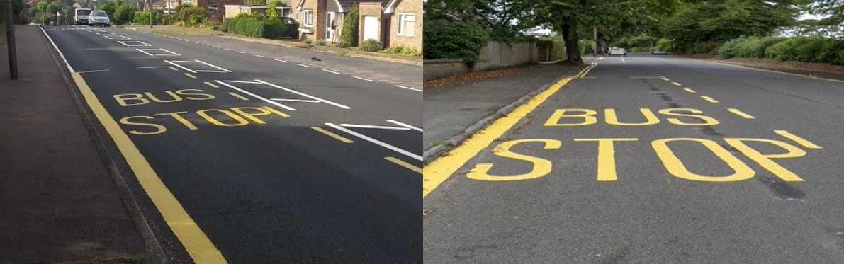
Bus Stops

The pavement space meant for bus stop is also marked by the word ‘BUS'(by yellow color).

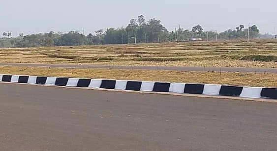
b. Kerb Marking

These may indicate certain regulations like parking regulations. Also the markings on the kerb and edges of islands with alternate black and white line increase the visibility from a long distance.

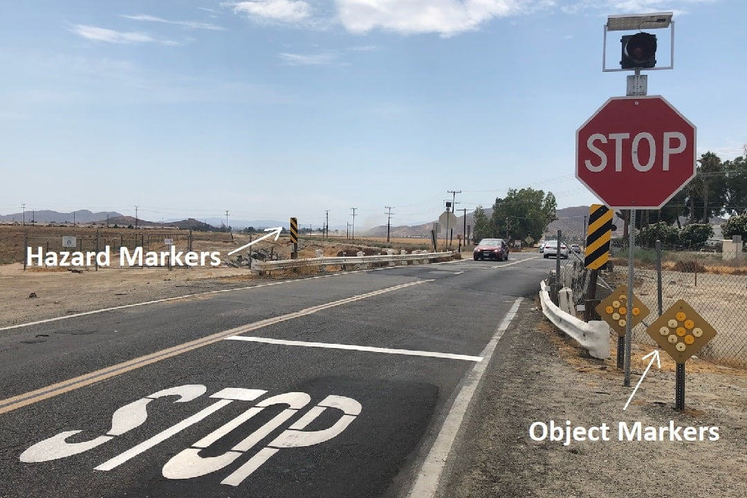
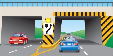
c. Object Marking

Physical obstruction on or near the roadway are hazardous and hence should be properly marked. Typical obstructions are supports for bridge, signs and signals, level crossing gates, traffic islands, narrow bridges, culver head walls etc.

d. Reflector Unit Marking

Reflector markers are used as hazard markers and guide markers for safe driving during night. Hazard markers reflecting yellow light should be visible from a long distance of about 150 m.

---

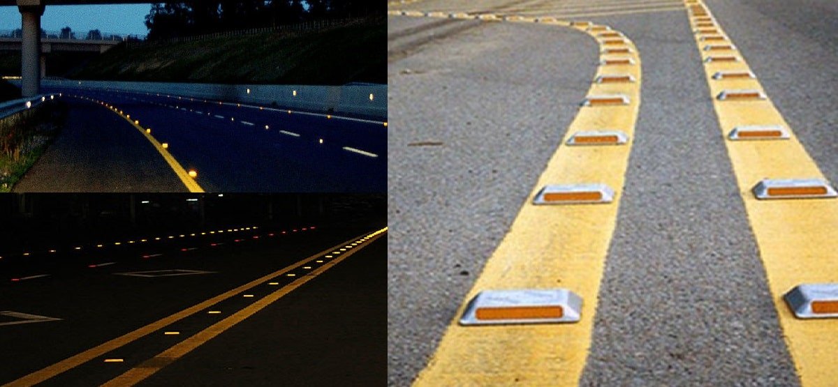
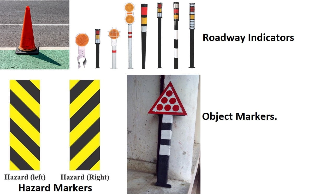
Road Delineators

Road delineators is provide visual assistance to drivers about the alignment of a road ahead, especially at night.

Reflectors are used on delineators for better nigh visibility.

Three types of Road delineators:

1. Roadway Indicators
2. Hazard Markers
3. Object Markers