Traffic Flow Characteristics & Capacity Study
- Traffic Capacity Studies
- Traffic Flow Characteristics Studies
⇓
1.Traffic Capacity Studies
Traffic Volume
Number of vehicle crossing the particular section of road is per unit time is called Traffic Volume. It is expressed in veh/day, veh/hr, veh/min.
Traffic Density (K)
Number of vehicle occupied by unit length of the road is called traffic density. It is expressed as vehicle/km, vehicle/metres.
Jam Density (Kj)
Traffic density under jam condition is called jam density. It is the maximum value of traffic density.
Note
- When density reaches to its maximum jam condition developed.
- Jam Condition is the worst condition on road under which congestion is so high, due to which movement of vehicle is not possible, hence speed of vehicle under jam condition is zero.
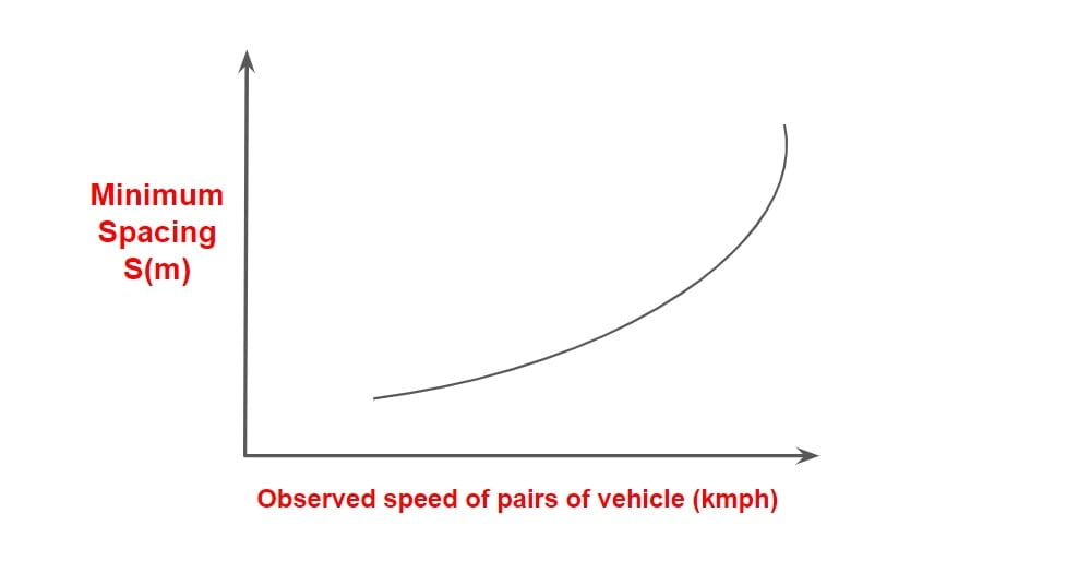
- Traffic Density varies with speed inversely, hence when with increase in speed of a stream vehicle on a roadway, the average density of vehicle decreases. This is because gap of spacing between the vehicle increases
 Space Headway (S)
- It is the distance, maintained between two consecutive vehicle travelling in same direction.

- It is the total length occupied by a moving vehicle on road, which includes length of vehicle and the gap between the two vehicle.
- This gap for safety point of view must be equal to SSD to avoid the collision between the two vehicle but this value of gap makes the designing over safe.
- Hence for geometric design this gap is computed by neglecting braking distance & considering reaction time to be 0.7sec instead of 2.5sec.
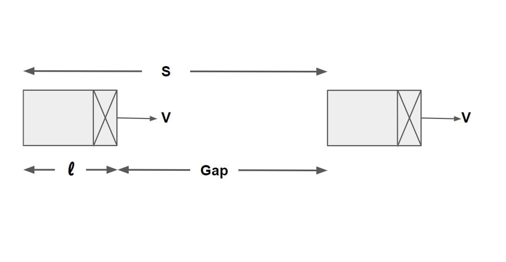
S= Gap + l.
(Gap ⇒ SSD)
we know that
SSD=\(0.278\times V\times tr\)+ \(\frac{V^{2}}{254(f±s \%)}\)
S = \(0.278\times V\times tr\)+ \(\frac{V^{2}}{254(f±s \%)}\) +l
neglecting braking distance & considering reaction time to be 0.7sec instead of 2.5sec
S = 0.278×tr×V + l
for geometric design, l= 6m, t= 0.7sec.
S = 0.278×0.7×V + 6
| S= 0.2V +6 | S= Space Headway in meter V= speed of vehicle in kmph |
Hence, Traffic density,
K = \(\frac{\text{1 (km)}}{\text{space headway (m)}}\)
K (veh/km)= \(\frac{1000}{\text{S (m)}}\)
| K (veh/km)= \(\frac{1000}{0.2V+l}\) | V→km/hr, l→meter, K → (veh/km) |
Note:
| Jam density Kj (veh/km)= \(\frac{1000}{l}\) | Under jam condition, V=0 (kmph) |
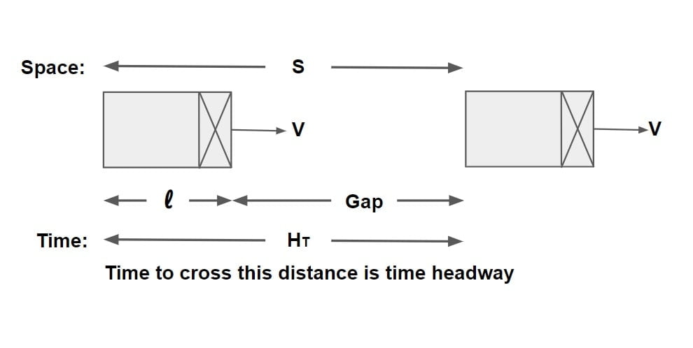
 Time Headway (HT)
It is define as the time gap between passing of two consecutive vehicle travelling in same direction.
 Traffic volume,
q= \(\frac{\text{1 hr}}{\text{average time headway}}\)
q (veh/hr)= \(\frac{3600}{{H_T (sec)}}\)
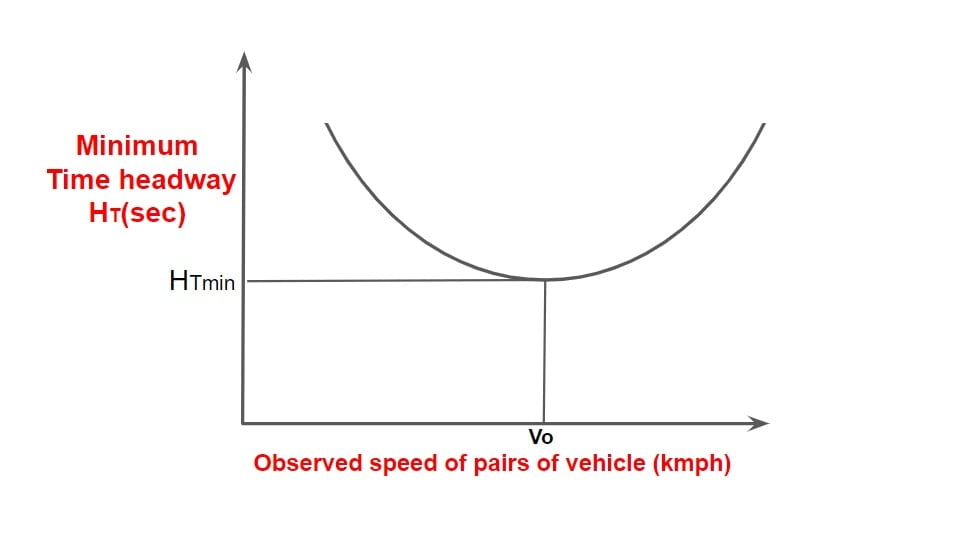
Note.1
- At very low speeds, the time headway is high and number of vehicle crossing a section on the road is also low. As speed of stream gradually increase, the minimum time headway decreases up to a lowest value at a certain speed.
- The speed at which the value of time headway is lowest represent the optimum speed corresponding max flow or capacity flow.
- If speed of traffic stream is further increased the minimum time headway starts increasing resulting in decrease of traffic flow.

Note.2
Relationship between traffic volume (q), Traffic density (K), and Traffic speed (V).
It is difficult to measure traffic density directly in practical situation, hence the relationship between traffic volume, traffic density and speed is used.
K (veh/km)= \(\frac{\text{q (veh/hr)}}{\text{V (km/hr)}}\)
| q= KV | Traffic volume = Traffic Density × Traffic speed |
| q (veh/hr) = \(\frac{1000}{\text{S (m)}}\) × V (km/hr) | we know that K (veh/km)= \(\frac{1000}{\text{S (m)}}\) |
also
q (veh/hr)= \(\frac{\text{3600}}{H_T (sec)}\)
From above two equation of q
\(\frac{3600}{H_T }\)=\(\frac{1000V}{\text{S }}\)
Traffic Capacity
Maximum value of traffic volume, which a road can accommodate is called Traffic Capacity. It is expressed as vehicle per hour per lane. (Traffic Volume ≤ Traffic Capacity).
Basic Capacity
This Traffic Capacity under most ideal condition is termed as Basic Capacity/Theoretical Capacity.
Note: Two road having the same physical features will have the same basic capacity irrespective of traffic condition, as they are assumed to be ideal.
Practical capacity
It is the maximum number of vehicle that can pass a given point on a roadway during one hour, without traffic density being so great, as to cause unreasonable delay, hazard or restriction to the driver’s freedom to maneuver under the prevailing roadway and traffic conditions.
Note:
- Sometimes practical capacity is also called as design capacity.
- For design purpose we neither use basic capacity or possible capacity as they represents the two extreme cases of roadway and traffic condition. Hence we have another type of capacity called Practical capacity.
Calculation of Theoretical Maximum Capacity
- Max Theoretical Capacity from Space Headway
- Max Theoretical Capacity from Time Headway
Max Theoretical Capacity from Space Headway
qmax = \(\frac{1000 V}{S}\)
Max Theoretical Capacity of lane,
C = \(\frac{1000 V}{S}\)
where,
C= Capacity of single lane (vehicle per hour)
V= speed of vehicle (kmph)
S= 0.2V +6 = Space Headway in meter
Max Theoretical Capacity from Time Headway
qmax= \(\frac{3600}{H_T}\)
Max Theoretical Capacity of lane,
C = \(\frac{3600}{H_T}\)
HT = Minimum time headway in seconds.
⇓
2.Traffic Flow Characteristics Studies
Traffic flow characteristics are divided under two categories:
- Macroscopic Characteristics
- Microscopic Characteristics
Macroscopic Characteristics
It represents how the behavior of one parameter of traffic flow changes with respect to another. There are many types of macroscopic models but we discuss only Green Shield’s Stream Model.
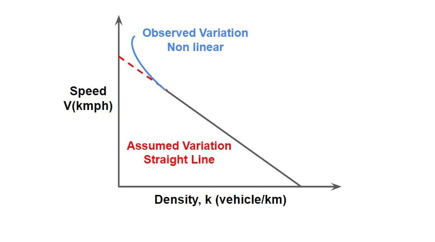
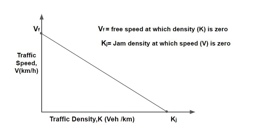
Green Shield’s Stream Model
Green shield’s assumed a linear speed- density relationship to derive this model.
 The equation for the relationship can be derived as
y= mx +c
V =mK +Vf
m = \(\frac{0-V_f}{Kj-0}\)
m = \(\frac{-V_f}{Kj}\)
V= Vf – \(\frac{V_f}{Kj}\)K
\(V=V_f\left ( 1-\frac{K}{K_j} \right )\)
This equation is referred as “Green Shield’s Stream Model”
now,
q= KV from previous relationship
q = \(V_f\left ( 1-\frac{K}{K_j} \right )\)K
q = \(V_f\times K-\frac{V_f\times K^{2}}{K_j}\)
using the above relationship, density can be found at which max flow occurs as follows
\(\frac{dq}{dK}=0\)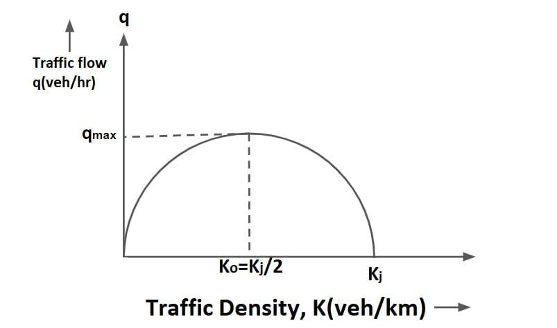
\(V_f-\frac{V_f\times (2K)}{K_j}\)=0
K= Kj/2
Density at which max flow occurs is denoted as optimum density,
KO= Kj/2
For qmax, put K=KO=Kj/2 in q
qmax = \(V_f\times \frac{K_j}{2}-V_f\times( \frac{K_j}{2})^{2}\cdot \frac{1}{K_j}\)
qmax = \(\frac{V_f\times K_j}{4}\)
since,
q = \(V_f\times K-\frac{V_f\times K^{2}}{K_j}\)
q= KV ⇒ K=q/V
q = \(V_f\times \frac{q}{V}-V_f\frac{q^{2}}{V^{2}K_j}\)
1 = \(\frac{V_f}{V}-\frac{V_f\times q}{V^{2}\times K_j}\)
\(V^{2}\times K_j=\frac{V_f\times V^{2}\times K_j}{V}-V_f\times q\).
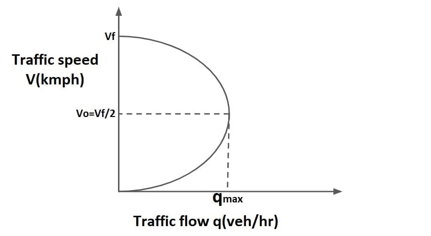
\(q= K_j\times V-\frac{K_j}{V_f}V^{2}\)to find the speed at which flow is max put K=KO=Kj/2
V= Vf – \(\frac{V_f}{Kj}\)K
at optimum speed V=VO, q=qmax
VO= Vf – \(V_f\frac{K_j}{2}\frac{1}{K_j}\)
VO= Vf /2
Microscopic Characteristics
In Microscopic Characteristics, we discuss about Time headway & Space headway. which already discussed.
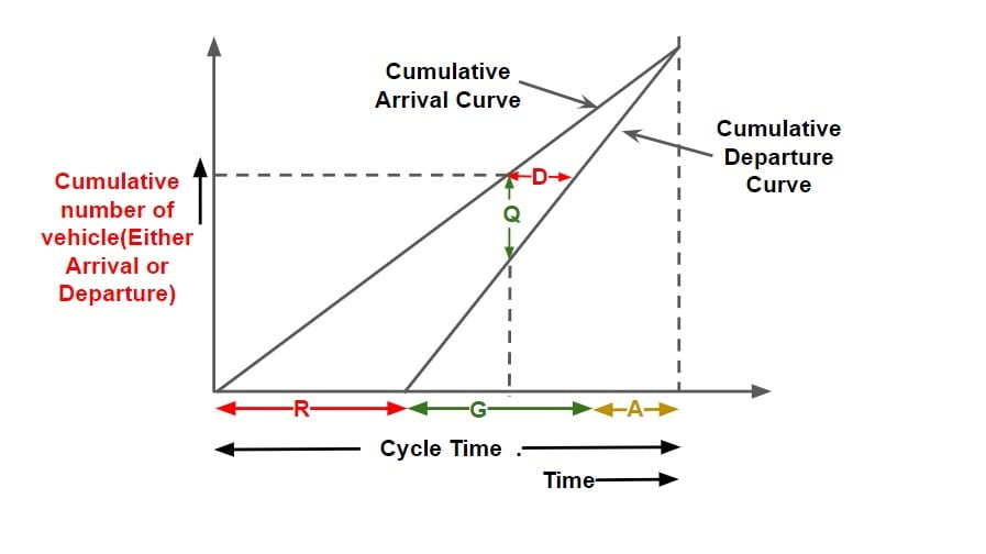
Delay & Queue Analysis at Signalized Intersection
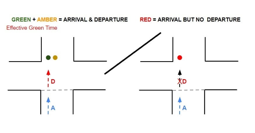
Delay (D)
- It is defined as the time a vehicle is stopped in queue while waiting to pass through signalized Intersection.
- It begins when the vehicle is fully stopped & end when the vehicle begin to accelerate.
- It is mathematically difference departure time & arrival time.
- Average delay is the average for all vehicle during the specified time period.
Queue (Q)
- It is the difference of total no of vehicle arrival & total number of vehicle departure at any instant of time.
 Note:
Note:
Average Delay Per Vehicle = {Area between cumulative arrival & cumulative departure curve for one cycle time } ÷ {Cumulative number of vehicle arrival per cycle time}
Assumption made in analysis
- Vehicle arrive & departure at uniform rate. (hence cumulative Arrival & cumulative departure curve with time is linear.)
- No pre existing queue is there at intersection.
- Arriving vehicle departs instantaneously when the signal is green.
- The departure of vehicle takes place at it max rate termed as Saturated Flow / Service Rate.
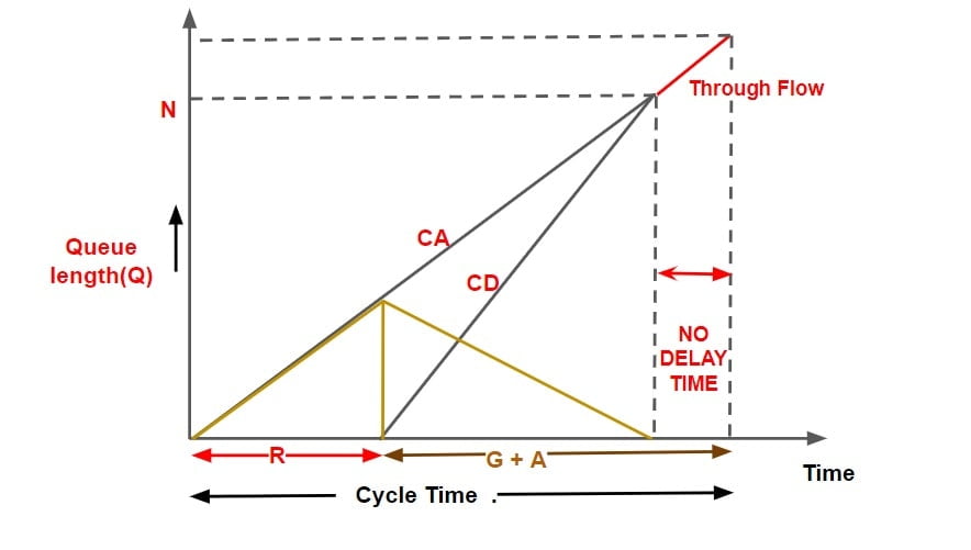
- The departure curve catches up with arrival curve before the next red interval begins.
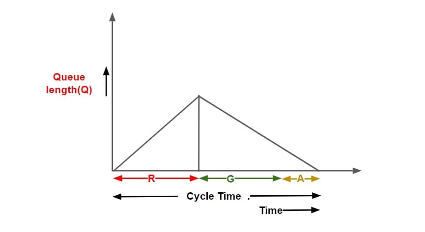
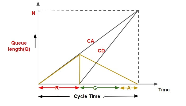
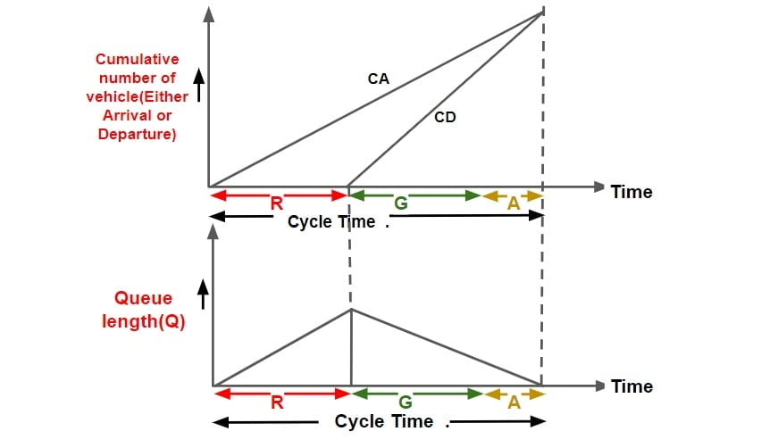 Note: Queue length v/s Time Graph can be converted into cumulative arrival & departure v/s time graph.
- Cumulative departure matches cumulative arrival exactly at the end of one cycle.

- Cumulative departure matches cumulative arrival before the completion of cycle time.

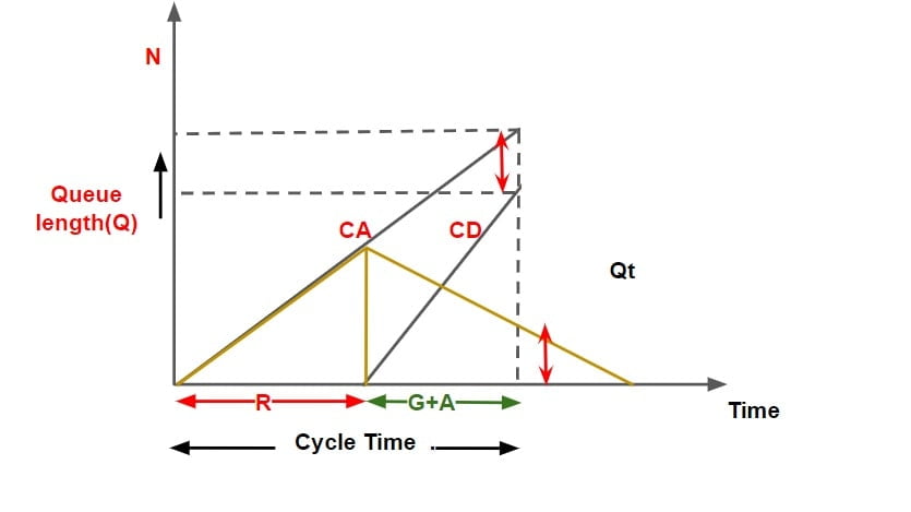
- Cumulative departure does not matches cumulative arrival even at the end of one cycle time.