Open Channel Flow – Introduction
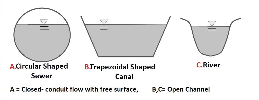
Open channel flow refers to the flow of liquid in a channel open to the atmosphere or a partially filled conduit (Pipe). Example- River, Flood, Rivulets, Torrent, Sewers carrying sewage, Rode side Gutter.
Note
- The free surface is an interface between the moving liquid and overlying fluid which will have constant pressure.
- In our case moving liquid is most of the time water and overlying fluid is air at atmospheric pressure (absolute pressure) or in terms of gauge pressure (0). (Gauge pressure = Absolute Pressure – Atmospheric Pressure)
- The driving force in OCF is gravity because all open channels have a bottom slope.
- Shear stress on the free surface is zero.
Difference Between Open Channel Flow and Pipe Flow
| Open Channel Flow | Pipe Flow | |
| 1 | OCF must have a free surface. | No free surface is available in pipe flow. |
| 2 | A free surface is subjective to atmospheric pressure. | No direct atmospheric pressure is available, only hydraulic pressure exists. |
| 3 | Here flow takes place due to gravity. | Here flow takes due to pressure difference. |
| 4 | Since gravitation force is governing force, here analysis is done by Froude’s Number. | Here analysis done by Reynold’s Number. |
| 5 | The depth of flow, discharge, and slope of the channel at the bottom and the free surface are interdependent. | Here there is no dependency between these parameter. |
| 6 | The cross-section may be of any form: circular, rectangular, triangular, or in the case of natural streams, it is irregular along the flow direction. | The cross-section of the pipe is generally kept circular. |
| 7 | In OCF depth of flow is variable so relative roughness changes with the level of the free surface. | The relative roughness is a fixed quantity. (Surface roughness varies with the type of pipe material) |
| 8 | HGL (Hydraulic Gradient Line) coincided with the free water surface. | HGL is usually above the conduit. |
Total Energy (ET) =Datum (Elevation) Energy + Pressure Energy + Kinetic Energy (velocity).
(The pressure energy is because of weight of water.)
ET = mgz + PV + ½·mv2
V=volume, v=velocity, m= mass, z= elevation, P= Pressure.
Head Form (Energy per unit weight): It is representation of energy in term of height of fluid column.
Energy/Weight (H) = Datum Head(z) + Pressure Head(P/γ) + Kinetic Head(v2/2g).
H= z + P/γ + v2/2g
H= z + hw + v2/2g
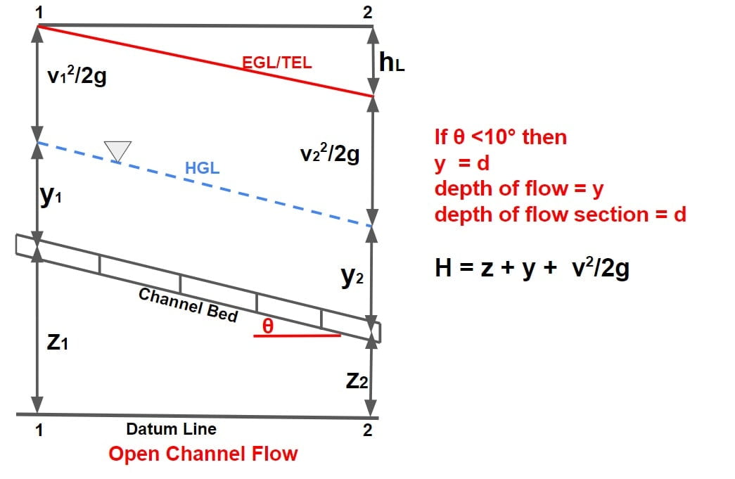
or H= z + y + v2/2g
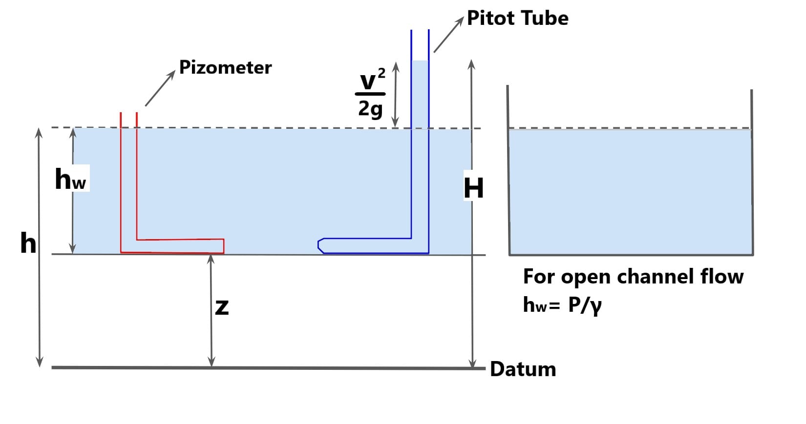
Note: Sum of datum head & pressure head is termed as hydraulic head (h). (Hydraulic head also called Piezometer Head)
h= z + P/γ
h= z + hw or h= z + y
hw or y= depth of flow (where the bed slope is between 0° to 10°),
h = hydraulic head or Piezometer Head,
z= datum head.
Note: here the bed slope is between 0° to 10°.
Hydraulic Gradient (i) = (Hydraulic head loss) / (Length of flow)
\(i= \frac{h_1-h_2}{L}\).
\(i= \frac{(z_1+h_{w1})-(z_2+h_{w2})}{L}\).
\(i= \frac{(z_1+y_1)-(z_2+y_2)}{L}\).
Energy Gradient (iE) = (Total head loss) / (Length of flow)
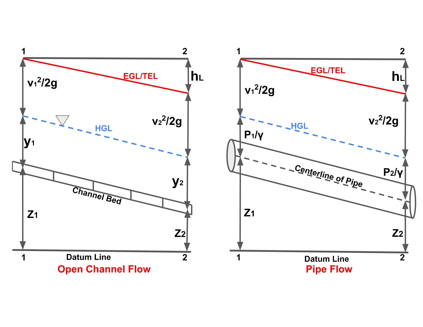
\(i_E= \frac{H_1-H_2}{L}\).
\(i_E= \frac{(z_1+\frac{P1}{\gamma }+\frac{v_1^{2}}{2g})-(z_2+\frac{P2}{\gamma }+\frac{v_2^{2}}{2g})}{L}\).
\(i_E= \frac{(z_1+y_1+\frac{v_1^{2}}{2g})-(z_2+y_2+\frac{v_2^{2}}{2g})}{L}\).
Line slope of which indicated hydraulic gradient is termed as HGL(Hydraulic Gradient Line).
Line slope of which indicated energy gradient is termed as TEL (Total Energy Line) or EGL (Energy Gradient Line).
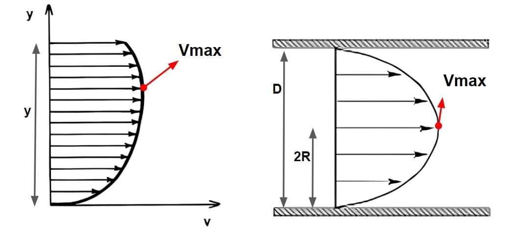
| 9 | The maximum velocity occurs at a little distance below the water surface. | The maximum velocity occurs at the center of the pipe. |
| 10 | Velocity distribution in case of ocf is logarithmic or power-law distribution. | In case of pipe flow velocity distribution is parabolic(for laminar flow.) |
Type of Force In Open Channel Flow
Different forces which may act over the fluid flowing in conduit are as follows.
- Inertia Force
- Gravity Force
- Viscous Force
Inertia Force
- It is the properties common to all the bodies that remain in their state, either rest or motion, unless some external cause in introduced to make them alter their state.
- It is product of mass & acceleration.
Fi = m·a = m·(v/t) = ρ·V·(v/t) = ρ·L3·(v/t)
Fi = ρ·L2·v2
m= mass, a= acceleration, v= velocity, V= volume, t= time, ρ= density, L= length .
Gravity Force
- It is a force due to own weight of the body/fluid.
Fg = m·g = ρ·V·g = ρ·L3·g
Fg = ρ·L3·g
ρ= density, L= length, g= acceleration due to gravity
Viscous Force
- This force is due to resistance of fluid against deformation which developed between different layer of fluid.
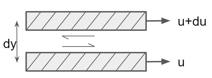
Fμ = τ·A
τ = μ · (du/dy) = μ · (v/L)
Fμ = μ · (v/L)·L2
Fμ = μ · v · L
τ = Shear stress, A= area, v= velocity, L= length, μ= coefficient of viscosity
Reynold’s Number
It is dimension less number that signifies the dominance of inertial force over viscous force.
It is the ratio of inertial force to the viscous force.
Re = \(\frac{F_i}{F_\mu } = \frac{\rho L^{2}v^{2}}{\mu vL} \)
Re = \( \frac{\rho vL}{\mu }\).
where:
- ρ is the density of the fluid (SI units: kg/m3)
- u is the flow speed (m/s)
- L is a characteristic linear dimension (m) (see the below sections of this article for examples)
- μ is the dynamic viscosity of the fluid (Pa·s or N·s/m2 or kg/(m·s))
Froude Number
It is dimension less number that signifies the dominance of inertial force over gravitation force.
Fr = \(\sqrt{\frac{\text{intertial force}}{\text{gravitation force}}}\)
Fr = \(\sqrt{\frac{\rho L^{2}v^{2}}{\rho L^{3}g}}\)
Fr = \(\frac{v}{\sqrt{gL}}\)
u = flow velocity, and L= characteristic length.
Different Types Of Open Channel
Open channel can be classified on the basis of following:
- On The Basis of Formation
- Natural Channel
- Artificial Channel
- On The Basis Of Change In Properties Of Channel
- Prismatic Channel
- Non Prismatic Channel
- On The Basis Of Type Of Boundary
- Rigid Boundary Channel
- Mobile Boundary Channel
1.On The Basis of Formation
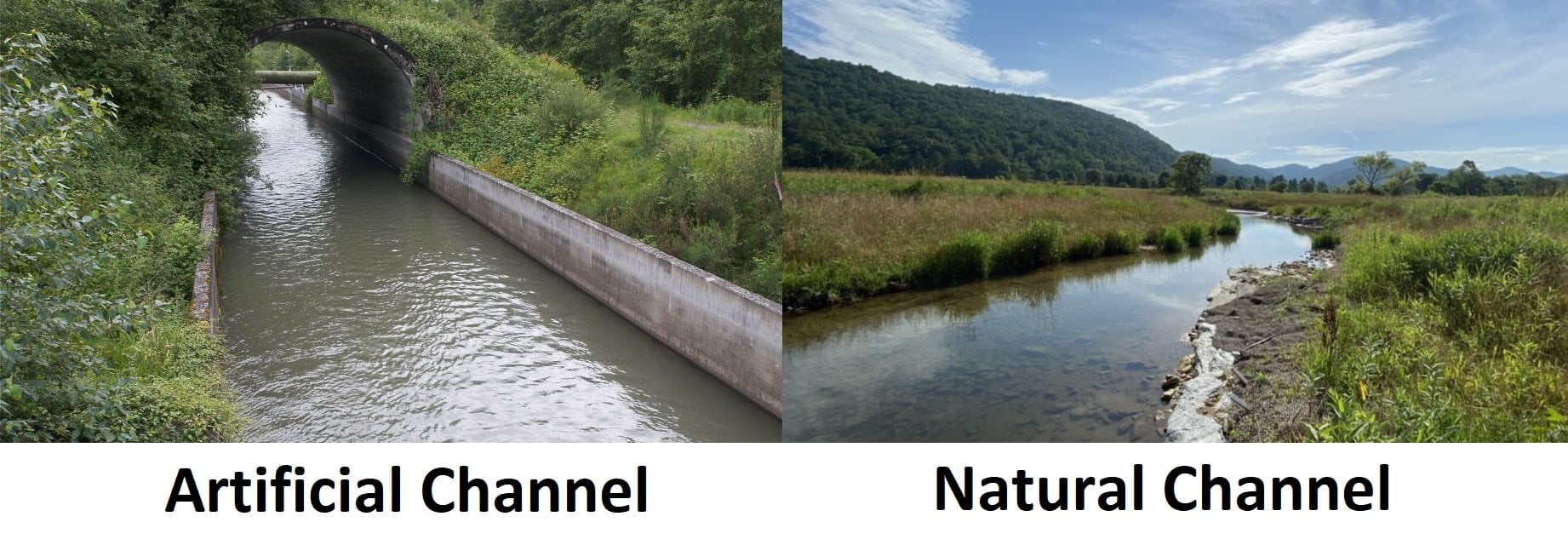
A. Natural Channel
- These are the channels which are formed by the action of natural force/act.
- They posses irregular geometry of cross section, planiform, depth of flow & bed slope.
- Example – River, Flood, Torrent, Rivulets, Creek, Road Side Gutter.
B. Artificial Channel
- The channels being constructed artificial to carry the water at desired operation in designed working condition are termed artificial channel.
- These channels are usually designed to have uniform cross-section, bed slope. depth etc.
- Example – Canals, Sewer, Open Flow Tunnel, Drop, Flume.
2. On The Basis Of Change In Properties Of Channel
A. Prismatic Channel
- A channel in which the cross section shape, size, bed slope, side slope, depth of channel (not depth of flow) are not change along the length is termed as a prismatic channel.
- Most of the man made channels are prismatic.
B. Non Prismatic Channel
- A channel in which any of the above three condition are not satisfied is know as non- prismatic channel.
- Mostly all natural channels are non prismatic.
3. On The Basis Of Type Of Boundary
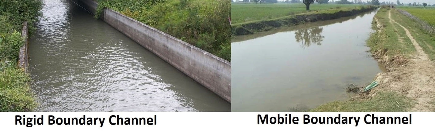
A. Rigid Boundary Channel
- Rigid channels are those in which the boundary is not deformable with the time. The shape and roughness factor is not a function of flow parameter.
- In other words, in Rigid channels, the flow velocity and shear stress distribution will be such that no major scouring, erosion or deposition will take place in the channel and the channel geometry and roughness are essentially constant with respect to time.
- For example, lined canals and non-erodible unlined canals.
- In rigid boundary channels only depth of flow vary with space & time depending upon nature of flow. Hence these channels have only One degree of freedom.
B. Mobile Boundary Channel
- These channels are those in which the boundary undergoes change, due to continuous erosion or deposition.
- In mobile channels, depth, bed width, bed slope and layout changes with space and time. Hence, these channels have four (4) degree of freedom.
Note: In the analysis open channel flow, channels considered would be artificial, prismatic & Rigid boundary channel.
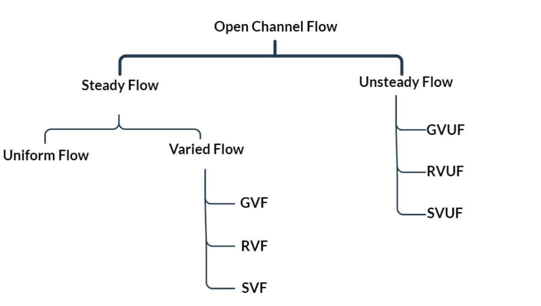
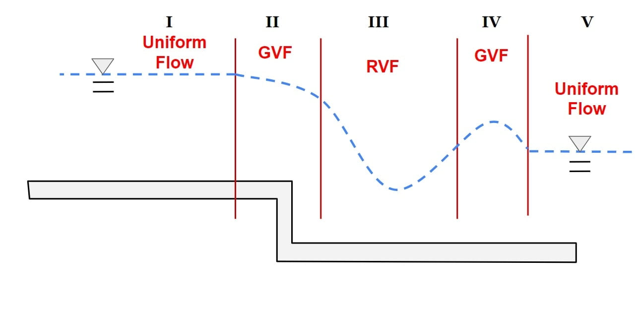
Types of Open Channel Flow
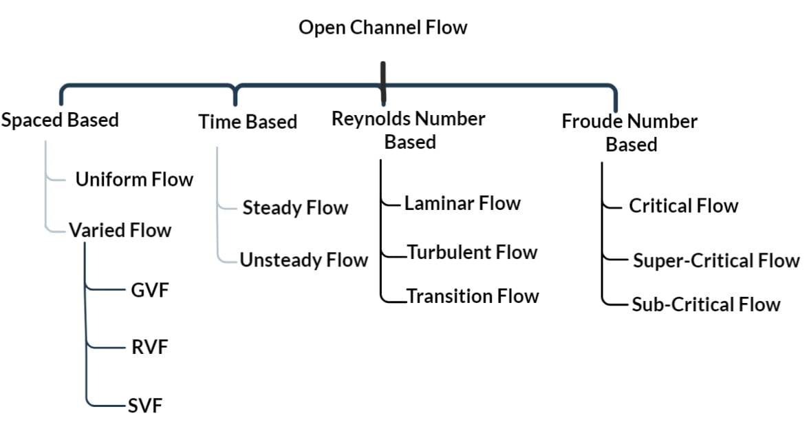
- Open Channel Flow
- Steady Flow
- Uniform Flow
- Non-Uniform Flow or Varied Flow
- Gradually Varied Flow
- Rapidly Varied Flow
- Spatially Varied Flow
- Unsteady Flow
- Gradually Varied Unsteady Flow
- Rapidly Varied Unsteady Flow
- Spatially Varied Unsteady Flow
- Steady Flow
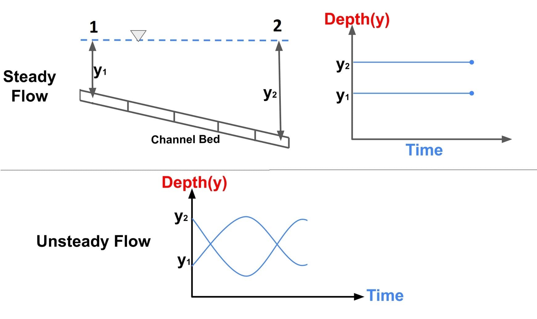
1. Steady & Unsteady Flows
- A steady flow occurs when the flow properties, such as the depth (y), velocity (v) or discharge (Q) at a section do not change with time at a fixed space.
\(\frac{dy}{dt}=0\).
\(\frac{dv}{dt}=0\).
\(\frac{dQ}{dt}=0\).
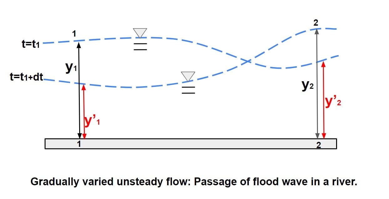
- If the properties of flow changes with respect to time at a fixed space are knows as unsteady flow.
\(\frac{dy}{dt}\neq0\).
\(\frac{dv}{dt}\neq0\).
\(\frac{dQ}{dt}\neq0\).
- Flood flows in rivers and rapidly varying surges in canals are some examples of unsteady flow.
 2. Uniform and Non-uniform flows
 2. Uniform and Non-uniform flows
- If the properties of flow do not vary with respect to space at any given instant of time is called uniform flow.
\(\frac{dy}{dx}=0\).
\(\frac{dv}{dx}=0\).
\(\frac{dQ}{dx}=0\).
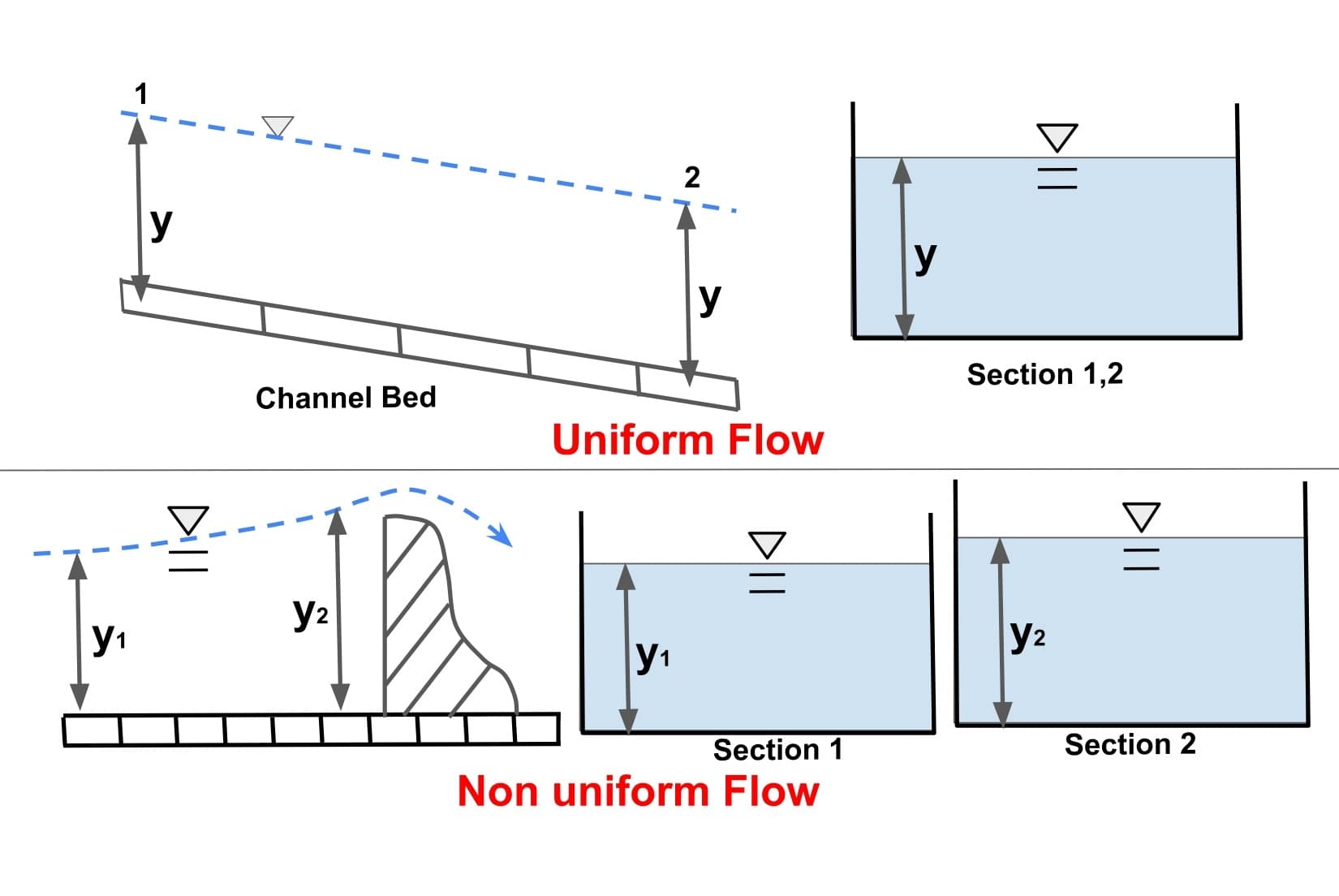
- If the properties of flow vary with respect to space at any given instant of time is called non uniform flow.
\(\frac{dy}{dx}\neq0\).
\(\frac{dv}{dx}\neq0\).
\(\frac{dQ}{dx}\neq0\).
Note: 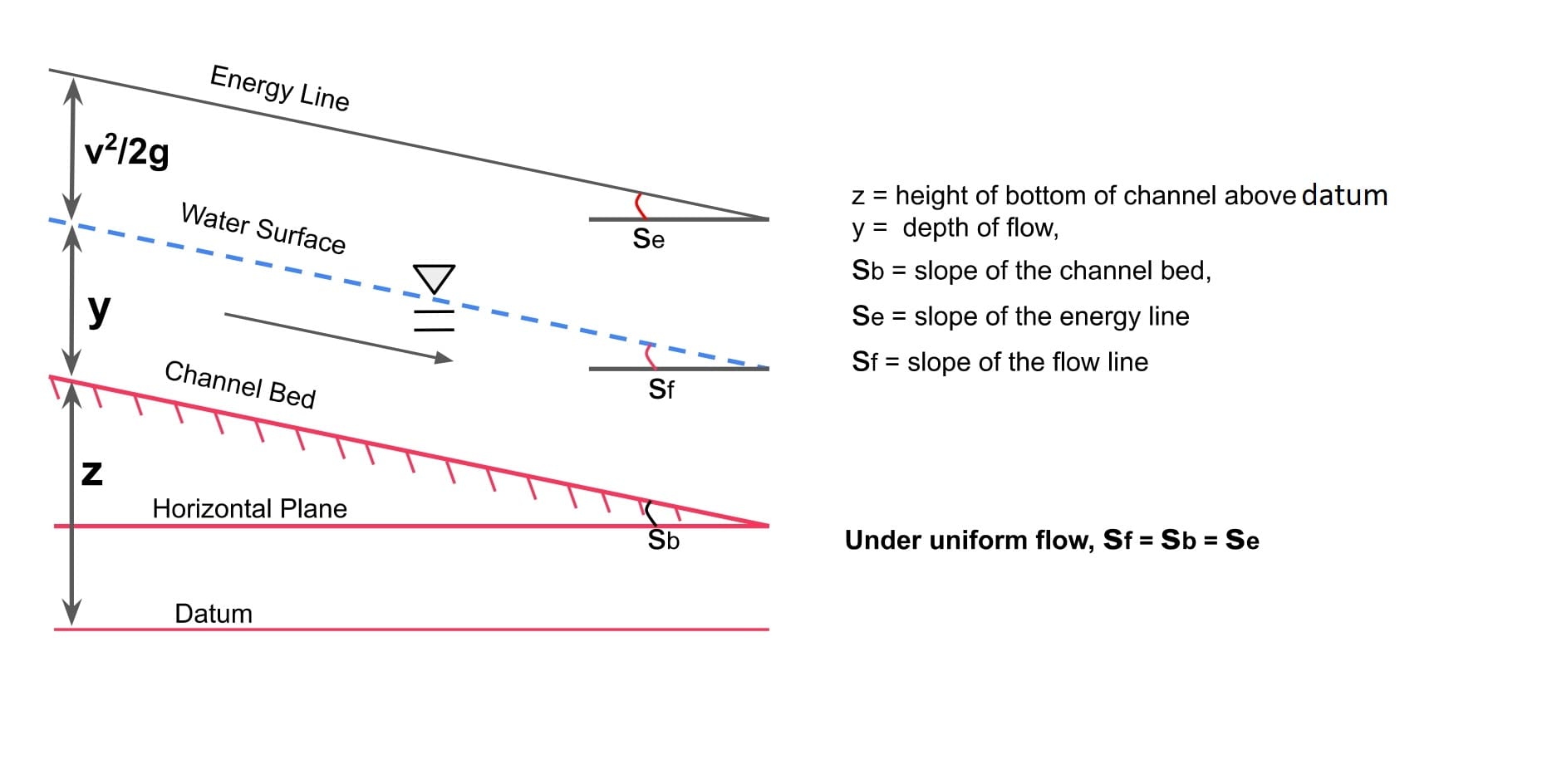
- Normal depth(y): The depth in uniform channel flow is known as normal depth.
- Under uniform flow, Bed slope = Energy line slope = Water surface slope
3. Varied Flow
- Flow in non- prismatic channel & flow with varying velocities in prismatic channel is termed as varied flow.
- As a uniform varied flow is not possible, this term is used only for non- uniform flow.
- Varied Flow is further classified as
- Gradually Varied Flow
- Rapidly Varied Flow
- Spatially Varied Flow
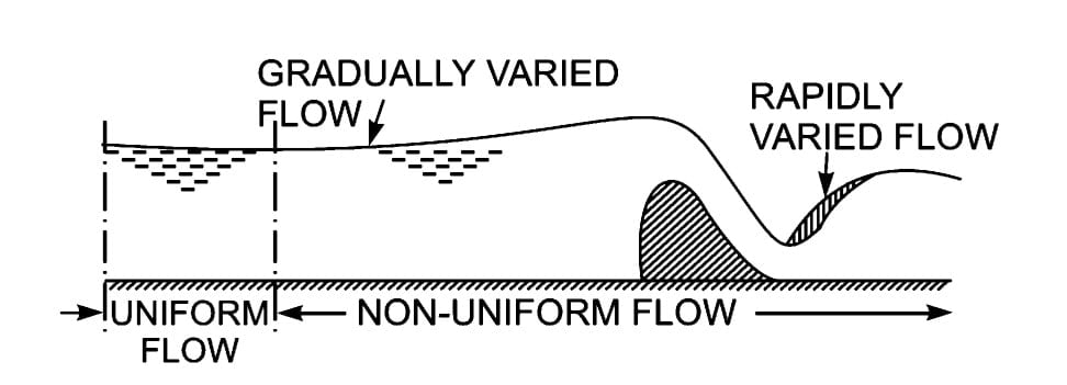
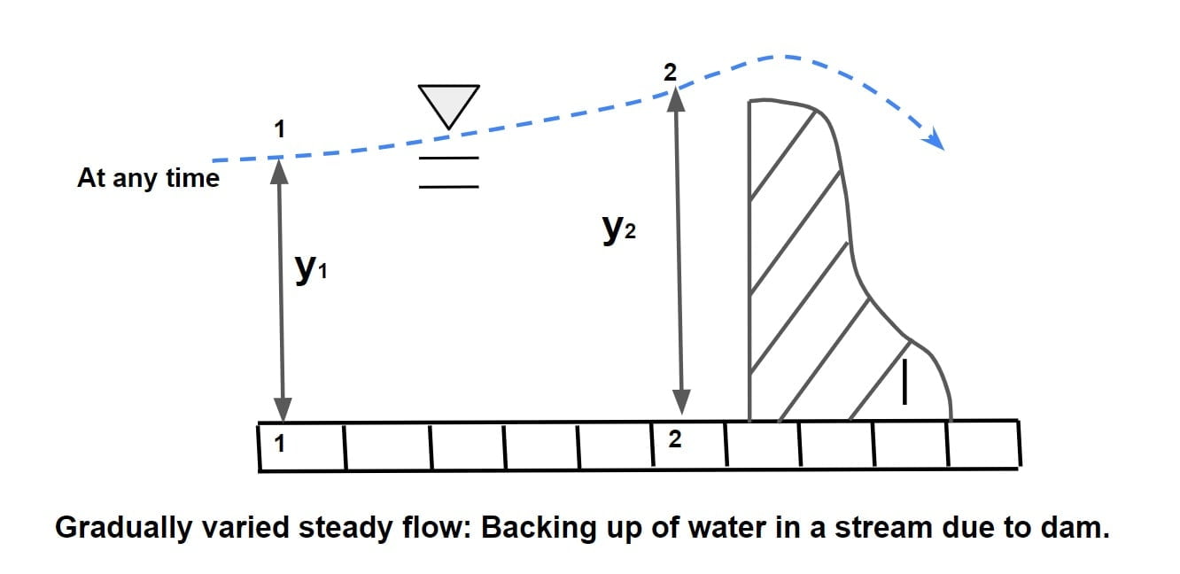
A. Gradually Varied Flow
- If the depth of flow changes gradually over the long distance along the length of channel such the curvature of free surface is mild, it is termed as Gradually varied flow.
- Example- Flow at upstream side of sluice gate.
- In GVF, loss if energy is mainly due to boundary friction.
- In GVF, the pressure distribution is vertical direction is taken hydrostatic.
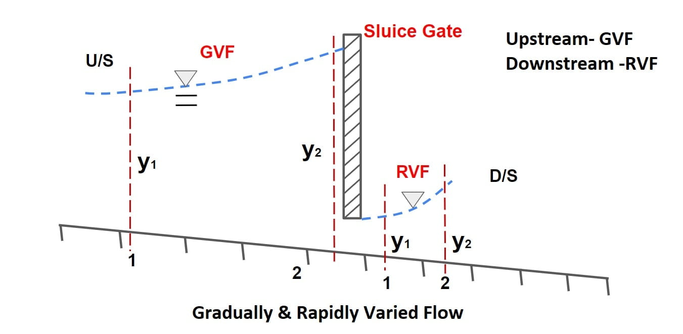
B. Rapidly Varied Flow
- If the depth of flow changes significantly over the short distance along the length of channel & curvature is large, it is termed as Rapidly varied flow.
- Example- Flow at downstream side of sluice gate.
- In RVF, frictional resistance are insignificant.
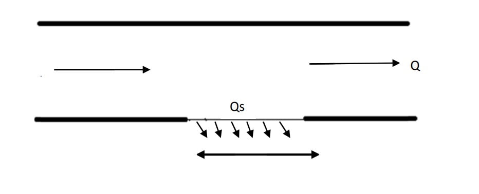
C. Spatially Varied Flow
- If some flow added or subtracted from the system then flow is called spatially varied flow.
- Example- Flow over a side weir, flow over a bottom rack, surface runoff due to rainfall is SVF.
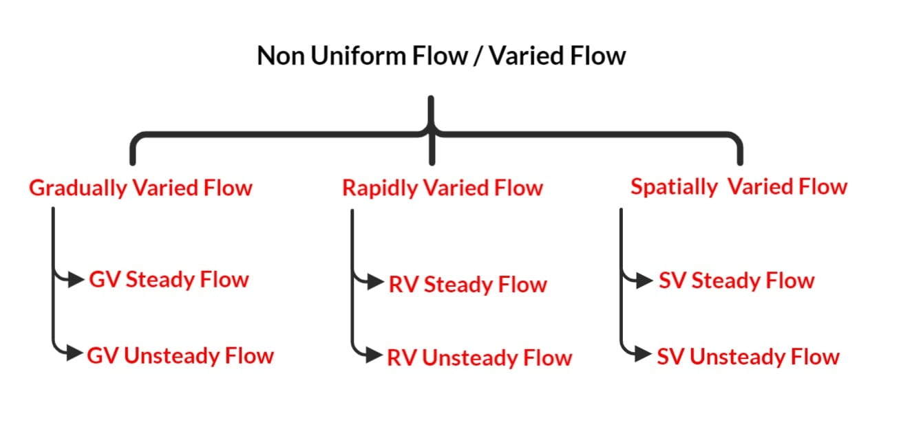
Types of Non-uniform flows Or Varied Flow
Gradually varied steady flow: Backing up of water in a stream due to dam.
Gradually varied unsteady flow: Passage of flood wave in a river.
Rapidly varied steady flow: A hydraulic jump below a spillway or a sluice gate.
Rapidly varied unsteady flow: A surge moving up a canal breaking of wave on the shore.
Spatially varied steady flow: Flow over side weir or flow over bottom rock.
Spatially varied unsteady flow: Surface runoff due to heavy rainfall.
Different Combination Of Flow
- Steady Uniform Flow: Possible
- Unsteady Uniform Flow: Not Possible
- Steady Non-Uniform Flow: Possible
- Unsteady Non-Uniform Flow: Possible
Note: If flow is uniform then it is always steady and if flow is non uniform it can be steady or unsteady.
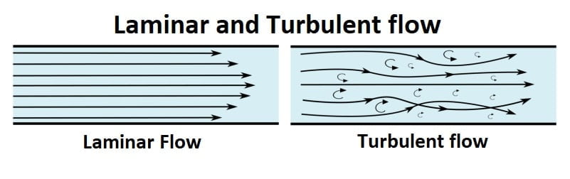
Laminar and Turbulent flow
Laminar Flow
- Laminar flow is defined as a fluid motion in which one layer slides over the other.
- Fluid particle of one layer does not go into the other layer i.e there is no momentum transfer between different layer.
- Generally laminar flow occurs at low velocity.
- In a highly viscous liquid, the flow is laminar.
- Near a solid border, the flow is laminar.
- In an open channel, Reynold’s Number must be less than 500 for the flow to be laminar. (Re<500)
Turbulent Flow
- Turbulent flow occurs when fluid particles flow in a highly disorganised manner, allowing particles from one layer to penetrate into another layer.
- In most cases, turbulent flow occurs at a high velocity.
- Momentum transfer continuous occur between the different layer.
- It occurs in fluid having low viscosity.
- In an open channel, Reynold’s Number must be greater than 2000 for the flow to be turbulent. (Re>2000).
Note:
- If properties of flow is in between laminar and turbulent, it is termed as transition flow.
- In open channel for flow to be transition 500<Re<2000.
Critical Flow, Subcritical Flow and Supercritical Flow
In case of open channel, since gravity force is governing force, analysis of this flow is done in terms of Froud’s Number instead of Reynold’s Number.
Here Froud’s Number used to differential between the critically of flow.
Fr = \(\sqrt{\frac{\text{intertial force}}{\text{gravitation force}}}\)
Fr = \(\sqrt{\frac{\rho L^{2}v^{2}}{\rho L^{3}g}}\)
Fr = \(\frac{v}{\sqrt{gL_c}}\)
Here Lc= characteristic length.
Characteristic length (Lc) for any cross sectional shape is expressed as
Lc = \(\frac{\text{area of flow}}{\text{Top width of flow}}\)
For example: If channel is rectanguler
Lc = \(\frac{A}{T}\)
Lc = \(\frac{By}{y}\)
Lc = y
Fr = \(\frac{v}{\sqrt{gy}}\)
At critical flow condition in Rectangular channel depth of flow is called critical depth (yc) and velocity of flow is called critical velocity (vc) and Froude number is equal to unity (1).
Fr = \(\frac{v}{\sqrt{gy_c}}\) =1
- If Fr <1: Flow is called sub critical.
- If Fr = 1: Flow is called critical. At critical flow condition specific energy a minimum.
- If Fr >1: Flow is called super critical or shooting flow or torrential flow called rapid flow.
| Type of flow | Depth Of flow | Velocity of Flow | Froude Number |
| Subcritical | y>yc | v<vc | Fr<1 |
| Critical | y=yc | v=vc | Fr=1 |
| Super critical | y<yc | v>vc | Fr>1 |
Celerity (Co)
Denominator of Froude number (\(\sqrt{gL_c}\)) represents the speed at which the disturbance wave travels in still water condition. It is called as celerity Co.
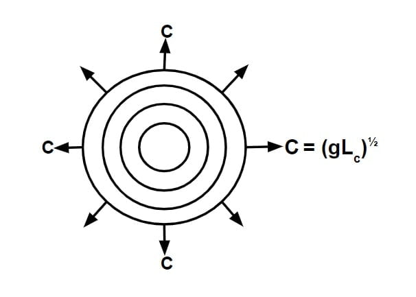 If we disturb the water which is not flowing, this disturbance wave occur & it propagates in all direction with a Celerity.
Co = (gLc)½
For a rectangular channel, Lc = y.
Hence celerity Co =\(\sqrt{gy}\)
Case.i
let flow is subcritical
Fr < 1
v <Co
- since v<Co, it can propagate both in upstream & down streams with a pattern as follows.
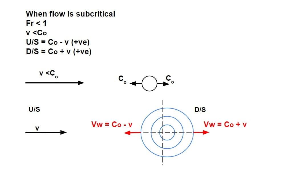
- This means the flow at upstream & downstream will be affected i.e there is hydraulic communication between upstream & downstream flow.
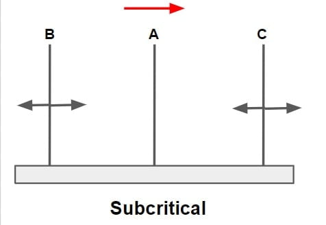
- Subcritical flows can be controlled from both upstream & downstream (i.e. downstream flow control)
Case.ii
let flow is critical
Fr = 1
v = Co
- since v = Co, it can propagate only in down streams direction with a pattern as follows.
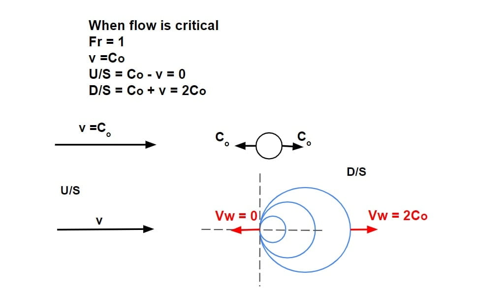
- This means the flow at downstream will be affected.
Case.iii
let flow is supercritical
Fr > 1
v >Co
- since v>Co, it cannot travel or propagate upstream, it can only propagate towards down streams with a pattern as follows
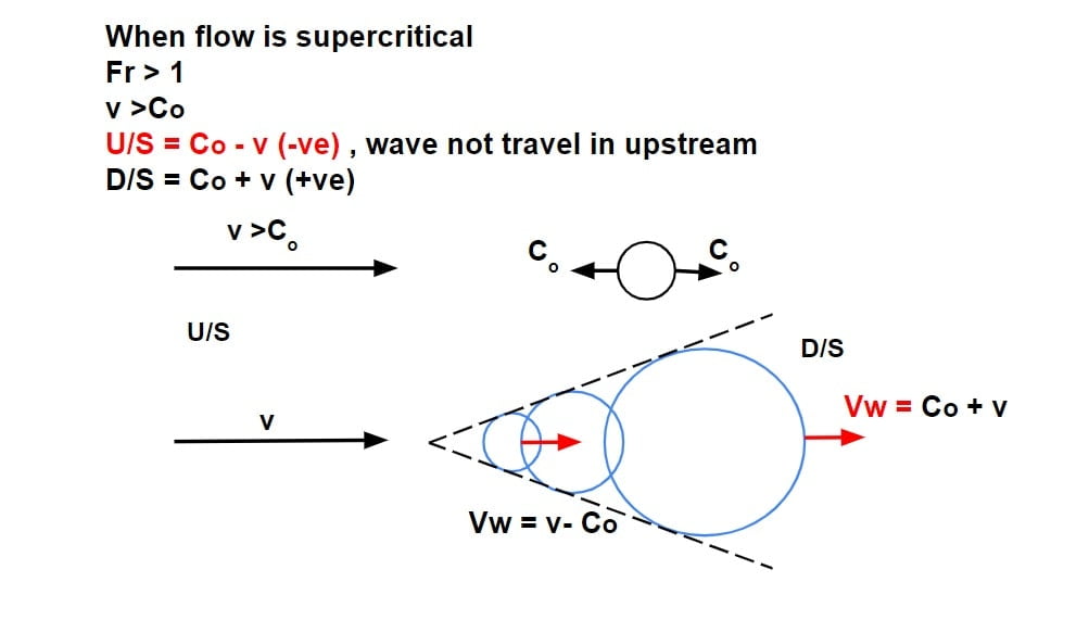
- It signifies that the flow at upstream will not be affected i.e there is no hydraulic communication between upstream & downstream flow.
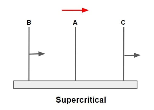
- A disturbance cannot travel upstream in a supercritical flow because the celerity is less than the flow velocity. Hence supercritical flows can only be controlled from upstream (i.e. upstream flow control)
Geometric Element Of Channel Section
- Depth of Flow (y)
- Depth of Flow Section (d)
- Top Width (T)
- Wetted/ Water Area (A)
- Wetted Perimeter (P)
- Hydraulic Radius/ Hydraulic Mean Depth of Flow (R)
- Hydraulic Depth
Depth of Flow (y)
It is the vertical distance of lowest point of channel section from the free surface.
Depth of Flow Section (d)
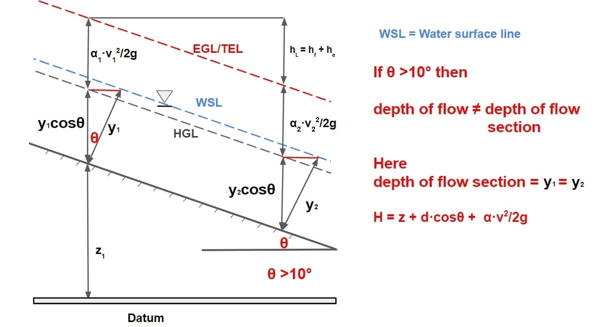
It is the normal distance of the lowest point of channel section from the free surface or it may also be termed as depth of flow normal to the direction of flow. (d = y·cosθ). . For most manmade and natural channels cosθ ≅1.0, and therefore y = d. The two terms are used interchangeably.
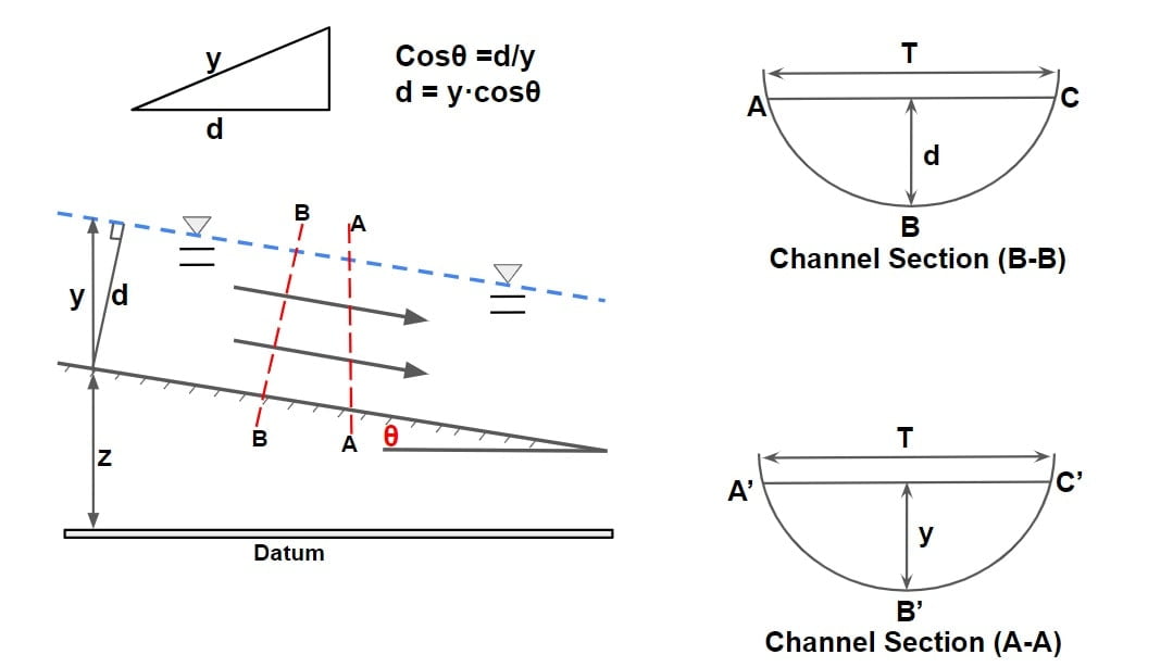
Top Width (T)
It is the width of the channel section at the free surface.
Wetted/ Water Area (A)
It is the cross section area of flow normal to the direction of flow.
Wetted Perimeter (P)
Length of the interface between the water and the channel boundary is called wetted perimeter. (Arc length of ABC)
Hydraulic Radius/ Hydraulic Mean Depth of Flow (R)
It is define as the ratio of water area to the wetted perimeter.
R = \(\frac{A}{P}\)
Hydraulic Depth
It is define as the ratio of the water area to the top width.
D = \(\frac{A}{T}\)

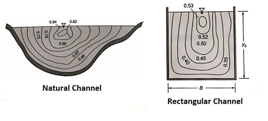
Velocity Distribution In Open Channel Flow
⇒ A typical velocity profile at a section in a plane normal to the direction if observed can be described by a logarithmic or power law distribution.
⇒ Velocity is zero at the boundaries & gradually increases with increases in distance from the boundary.
⇒ This distribution is quite non-uniform due to
- Non uniform shear stress along wetted perimeter.
- Presence of free surface on which the shear stress is zero.
⇒ It has been observed that maximum velocity of flow occurs at certain distance below the free surface. This reduction is due to the production of secondary current which is the function of aspect ratio (ratio of width to depth B/y).
⇒ The presence of corners, boundaries & bends in open channel cause the velocity vectors of flow to have compound not only in longitudinal but also in lateral & normal direction.
⇒ This flow in normal direction is secondary flow & produces secondary currents.
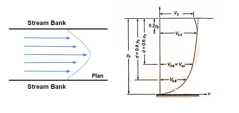
Top view of stream bank, don’t confuse.
Note: Contour of equal velocity are called as “ISOVELS”.
 ⇒ From the field observations, it has been observed that average velocity of flow occurs at a depth 0.6yo from the free surface, where yo = depth of flow.
vavg= v0.6. (Less reliable)
⇒ In deep channels however the above relation is unreliable hence average velocity is taken to be average of flow at 0.2yo & 0.8yo from free surface.
vavg = \(\frac{v_{0.2y_o}+v_{0.8y_o}}{2}\)
Average velocity is also related to surface velocity as
vavg = K·vs
vs = Surface velocity
K= 0.8 to 0.95
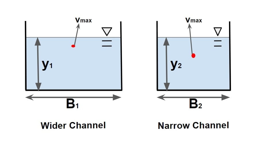
⇒ Note: For deep narrow channels, the location of maximum velocity point will much lower from the water surface than for a wider channel & same depth.
Wider channel dip will be insignificant. for wider channel B/y o≥ 5.
Narrow channel dip will be significant. for narrow channel B/y o≤ 5.
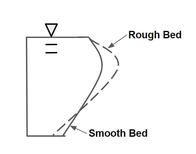
Note:
- The roughness of the channel will be affect the curvature of the vertical velocity distribution curve & tends to increase it.(If roughness increase than curvature of velocity distribution is increase.)
 Surface wind very little effect over Velocity distribution.
 Surface wind very little effect over Velocity distribution.
Average velocity of the channel can also be represented as
Average velocity, V= \(\frac{1}{A}\int_{A}^{}v\cdot dA\) (in the form of actual velocity)
As per conservation of mass
Q= constant
Q= AV
V=\(\frac{1}{A}\int_{A}^{}vdA\)
Q= AV= \(\int_{A}^{}vdA\)
v= actual velocity
V= average velocity
Kinetic energy correction factor (α)
It is ratio of kinetic energy of flow per second based on actual velocity to the kinetic energy of flow per second based on average velocity.
α= \(\frac{\frac{1\cdot m\cdot v_{act}^{2}}{2\cdot t}}{\frac{1\cdot m\cdot v_{avg}^{2}}{2\cdot t}}\).
| numerator of α |
| \(\frac{1\cdot m\cdot v_{act}^{2}}{2\cdot t}\) mass(m) =density(ρ)×volume \(\frac{1\cdot \rho \cdot volume\cdot v_{act}^{2}}{2\cdot t}\) volume/t=Q(discharge) \(\frac{1\cdot \rho \cdot Q\cdot v_{act}^{2}}{2}\) Q= AV= \(\int_{}^{}vdA\) \(\frac{1\cdot \rho \int v_{act}\cdot dA\cdot v_{act}^{2}}{2}\). \(\frac{1\cdot \rho \int dA\cdot v_{act}^{3}}{2}\). vact=v. |
| denominator of α |
| \(\frac{1\cdot m\cdot v_{avg}^{2}}{2\cdot t}\) mass(m) =density(ρ)×volume \(\frac{1\cdot \rho \cdot volume\cdot v_{avg}^{2}}{2\cdot t}\) volume/t=Q(discharge) \(\frac{1\cdot \rho \cdot Q\cdot v_{avg}^{2}}{2}\) Q= AV (V=avg velocity ) \(\frac{1\cdot \rho \cdot A \cdot v_{avg} \cdot v_{avg}^{2}}{2}\). \(\frac{1\cdot \rho \cdot A \cdot v_{avg}^{3}}{2}\). vavg = V. |
So Kinetic energy correction factor (α) can be represented as
α= \(\frac{\int_{}^{}v^{3}dA}{V^{3}A}\)
α= coriolis coefficient
v= actual velocity
V= average velocity
Momentum correction factor (β)
It is ratio of momentum of flow per second based on actual velocity to the momentum of flow per second based on average velocity.
β= \(\frac{\frac{ m\cdot v_{act}}{t}}{\frac{m\cdot v_{avg}}{ t}}\).
| numerator of β |
| \(\frac{ m\cdot v_{act}}{t}\) mass(m) =density(ρ)×volume \(\frac{\rho \cdot volume\cdot v_{act}}{ t}\) volume/t=Q(discharge) \(\rho \cdot Q\cdot v_{act}\) Q= AV= \(\int_{}^{}vdA\) \(\rho \cdot \int_{}^{}v_{act}dA\cdot v_{act}\) \(\rho \cdot \int_{}^{}v_{act}^{2}\cdot dA\) vact=v. |
| denominator of β |
| \(\frac{ m\cdot v_{avg}}{t}\) mass(m) =density(ρ)×volume \(\frac{\rho \cdot volume\cdot v_{avg}}{ t}\) volume/t=Q(discharge) \(\rho \cdot Q\cdot v_{avg}\) Q= AV (V=avg velocity ) ρ·A·V·V = ρ·A·V2 vavg=V. |
So Momentum correction factor (β) can be represented as
β= \(\frac{\int_{}^{}v^{2}dA}{V^{2}A}\)
β= boussinesq coefficient
Values of α and β
- Generally, α > β> 1
- In case of uniform velocity distribution, α = β= 1
- Large and deep channels with regular cross section and fairly straight alignment have lower values of α and β, compared to smaller channels with regular cross section.
Pressure Distribution
Case (i) Channel With Small Slope
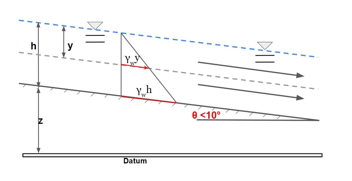
⇒ If slope of channel is very small (in the range of <10°) for such channels the vertical section is partially same as that the normal section. {depth of flow (y)≈ depth of flow section(d)}
⇒ If flow takes in this channel with the water surface parallel to bed i.e uniform flow, in such case streamlines will be straight line and it can be referred that depth of flow(y) would be equal depth of flow section(d).∴ d = y·cosθ
θ <10°
d=y
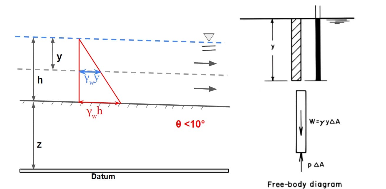
ΣFy =0
weight of water = PΔA
ρgyΔA = PΔA
or
p = ρgy = γy
⇒ Thus the piezometric head at any point in this channel will be equal to water surface elevation, hence HGL coincides with water surface.
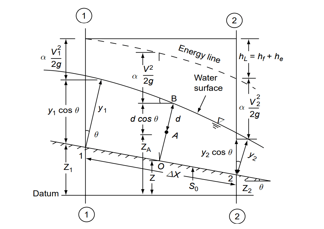
Case (ii) Channel With Large Slope
⇒ If slope of channel is very large (in the range of >10°).
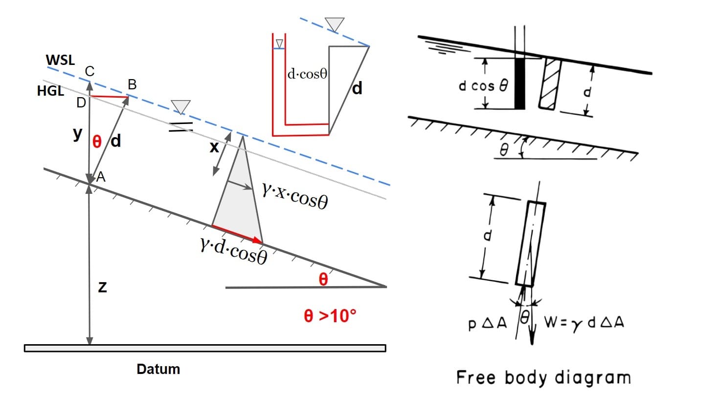
If θ = slope of the channel bottom, then the component of the weight of column acting along the column is ρgdΔA cos θ and the force acting at the bottom of the column is pΔA
ΣFy =0
weight of water × cosθ = pΔA
ρgdΔA×cosθ = pΔA
or
p = ρgd·cosθ
p= γd·cosθ
By substituting d = y cos θ (from ΔABC)into this equation (y = flow depth measured vertically)
p = γy cos2θ
Note:
Piezometric height at bottom = z+d·cosθ
water surface level at point c = z+ y
(d·cosθ<y)
(d·cosθ =AD, y=AC from image)
Hence in this case it can be concluded than HGL does not lie on water surface level. For large slope HGL will below the free surface.
Conclusion Pressure at any point in Open Channel flow for any Slope p = γ·y ·cos2θ p = γ·d ·cosθ y = vertical depth or Depth of Flow d= normal depth or depth of flow section |
Different Equation Used In OCF
- Continuity Equation
- Energy Equation
Momentum Equation
1.Continuity Equation
- It is based on conservation of mass.
- In OCF, since incompressible fluid are analyzed this equation is relatively easy to use.
(A). Continuity Equation For Steady Flow (Uniform Flow, GVF, RVF)
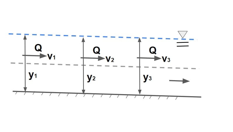
- In a steady flow the volumetric rate of flow (Q) through any section is same.
- Then for section having different areas Q = AV= A1V1 = A2V2 …………= AnVn.
(B). Continuity Equation For Steady Flow (SVF)
- In a steady spatially varied flow, the discharge at various section will not be same.
- In such the case following change in the analysis is done.
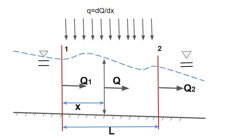
Let rate addition of water/ discharge be q
q= \(\frac{dQ}{dx}\).
Then discharge at distance ‘x’ from section 1.
Q= Q1 + \(\int_{0}^{x}q\cdot dx\)
let q = constant
Q= Q1 + q·x
Hence continuity equation for steady spatially varied flow is give by
q= ± \(\frac{dQ}{dx}\).
(C). Continuity Equation For Unsteady Flow (GVF, RVF)
- Due to unsteady flow discharge are not same with respect to time. So Q2> Q1 ,more water goes out than water coming into section 1-1.
- The excess volume of outflow in time Δt is computed by considering the depletion of storage within the control volume due to which water surface start falling.
- Here, we can also say that
\(\frac{\partial Q}{\partial x}= \frac{Q_2-Q_1}{\Delta x}\)
Q2 – Q1 = \(\frac{\partial Q}{\partial x} \Delta x\).
Net quantity of water leaving the system in Δt
ΔV =(Q2 – Q1)· Δt = \(\frac{\partial Q}{\partial x} \Delta x\)· Δt………(1)
Rate of depletion of water in control volume in Δt
ΔV = \(\frac{\mathrm{d} (dA\Delta x)}{\mathrm{d} x}\Delta t\)
ΔV = \(\frac{\mathrm{d} (Tdy\Delta x)}{\mathrm{d} x}\Delta t\)………(2)
as per continuity equation 1=2
\(\frac{\partial Q}{\partial x} \Delta x\)· Δt=-\(T\frac{\mathrm{d} y}{\mathrm{d} x}\Delta x\Delta t\)
\(\frac{\partial Q}{\partial x} \) +\(T\frac{\mathrm{d} y}{\mathrm{d} x}\)=0
Note: Continuity Equation of Unsteady Spatially Varied Flow is
\(\frac{\partial Q}{\partial x}\) +\(T\frac{\mathrm{d} y}{\mathrm{d} x}\)= ±q
2.Energy Equation
⇒ In the one-dimensional analysis of steady open-channel flow, the energy equation in the form of the Bernoulli equation is used.
⇒ According to this equation, the total energy at a downstream section differs from the total energy at the upstream section by an amount equal to the loss of energy between the sections.
Total Energy (in head form) = Datum Head + Pressure Head + Kinetic Head.
H = z + P/γ + v2/2g
H = z + y + v2/2g
H= Total Head (total energy/weight)
z= Datum Head, P/γ or y =Pressure Head, v2/2g =Kinetic Head
Total Energy in term of Pressure
Total Energy (in pressure form) = γ·z + P + ρ·v2/2
γ·z = Hydrostatic Pressure, P= Static Pressure, ρ·v2/2 = Dynamic Pressure.
Note:
⇒ Sum of datum head & pressure head is termed as hydraulic head (h). (Hydraulic head also called Piezometer Head)
h= z + P/γ
Stagnant Head = v2/2g + P/γ
⇒ In steady varied flow in a channel. If the effect of the curvature on the pressure distribution is neglected (P/γ=depth of normal flow (d) in open channel), the total energy head is given by
H = z + d·cosθ + α·v2/2g
At any two given section 1-1 & 2-2 as per Bernoulli’s Equation
z1 + y1·cosθ + α1·v12/2g = z2 + y2·cosθ + α2·v22/2g + hL
or H1-H2= hL
Note
- If the channel bed slope comparatively small (θ <10°) than cosθ=1.
- If the flow take place in deep, wide, smooth turbulent channel the value of α≅1.
- Here total head loss between any two section (hL) consist of friction head loss (hf) + eddy head loss(he). {hL = hf + he}
- For prismatic channels, head loss due to eddy’s is zero (he =0).
- The slope of energy line depends on roughness characterizes and change in properties of channel section.
- Slope of hydraulic gradient line depends type of flow & slope of channel bed.
- The bed slope of geometric parameter of channel.
- At any given in open channel, slope of total energy line, channel bed& hydraulic gradient is different.
3.Momentum Equation In Open Channel Flow
⇒ Momentum is a vector quantity. The momentum equation commonly used in open channel flow problems is the linear-momentum equation.
⇒ According to Newton’s second law of motion, the rate of change of momentum is equal to the resultant of all the external force acting on the body.
Steady flow
⇒ In steady state, the rate of change of momentum in a given direction will be equal to the net flux of momentum in that direction.
Note: Force generally acting on fluid mass.
- Pressure force acting on control surface.
- Friction force acting on channel bed.
- Body force (component of self weight of fluid mass) in direction of flow.
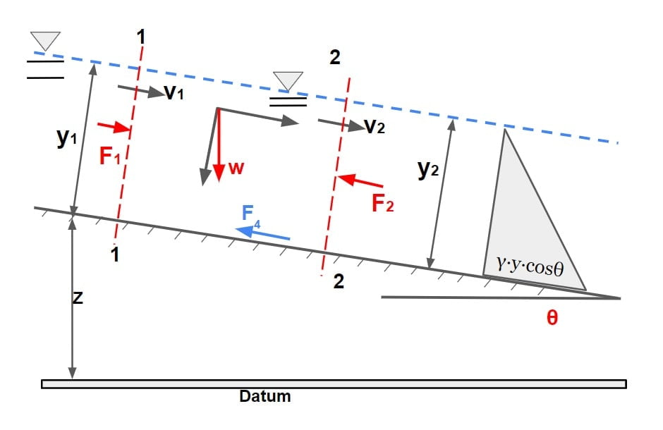
F1 + F3 – F4 – F2 = M2 – M1
F1 & F2= Pressure force acting at section 1 & 2 respectively
F= pressure × area
(pressure in open channel flow is not uniform along the depth so for calculating force , pressure taken as average pressure)
p= (o+ρ·g·y·cosθ)/2
p= \(\frac{\rho \cdot g\cdot y\cdot cos\theta }{2}\)
ρ= density, A= area of flow section,
F= \(\frac{\rho \cdot g\cdot y\cdot cos\theta }{2}(y\cdot B)\)
NOTE: (here y is normal depth not vertical depth)
F3= Force due to weight of water in the direction flow.
F3=w·sinθ
F4 =Total external force of friction or resistance acting along the surface of contact between the water and the channel.
M1 & M2= momentum per unit time at section 1 & 2 respectively or momentum flux
momentum per unit time = m·v/t
m=ρ·V , ∴{density (ρ) = mass (m) / volume (V)}
V/t = Q, ∴{Discharge= Volume/time}
M1 = β1·ρ·Q·v1
M2=β2·ρ·Q·v2
β = Momentum correction factor.
for turbulent flow,
β1 = β2= 1
Un-steady flow
- In unsteady flow, momentum equation states that the algebraic sum of all the external forces on a fluid mass in the direction of flow is equal rate of change of momentum in direction of flow + the time rate of increase of momentum in the same direction within control volume.
SPECIFIC FORCE
⇒ Specific force is the sum of pressure force and momentum flux per unit “unit weight” of the fluid at a section.
⇒ The steady state momentum equation takes a simple form, if the channel is assumed to be horizontal and frictionless.
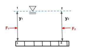
M2 – M1 = F1 – F2
As channel is assumed frictionless and bed is horizontal w·sinθ=0
M1 + F1 = F2 + M2
\(\frac{F_1+M_1}{\gamma _1}=\frac{F_2+M_2}{\gamma _2}\)
\(\frac{F+M}{\gamma}= \text{Specific Force}\)Note:
- Specific force for horizontal frictionless channel will be constant.
- In the analysis of rapidly varied flow, friction not play a significant role hence for small slope of bed RVF analysis id done by making the specific force to be constant.
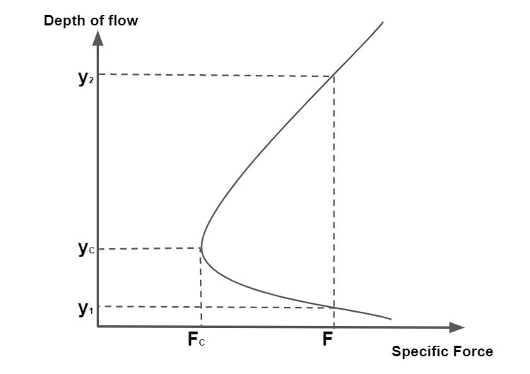
The specific force for a given discharge is minimum when the flow is critical (Fc = 1.0). At a value of F> Fc, there are two depths of flow y1 and y2 which yield the same specific force at the given discharge. These depths are called conjugate depths or sequent depths.
og content bro