Pavement Design: Introduction  

• Pavement is a load-bearing & load-distributing component of a road.
• We need to consider all types of vehicles for the geometrical design, but only vehicles with significant heavy loads are considered for pavement design.
• These vehicles are generally commercial vehicles.
• As per IRC, vehicles having a gross load greater than 3 tons are called commercial vehicles.

  Types of Pavement in Highway Engineering

Pavements can be classified as follows:

• Flexible Pavement
• Rigid Pavement
• Semi- Rigid Pavement
• Composite Pavement

Flexible Pavement

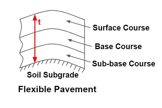
1. The pavements which have very less flexural strength are called flexible pavement.
2. A flexible pavement is one that is made up of one or more layer of materials, the highest quality material forming the top layer.
3. The load carrying capacity of the flexible pavement is derived from the load distribution properties & not from its flexural strength.
4. The flexible pavement layer reflects the deformation of the lower layer. Thus if lower layer of pavement of soil subgrade is undulated, the pavement surface also gets undulated.
5. This type of pavements transmit the load to the lower layer by grain to grain transfer.
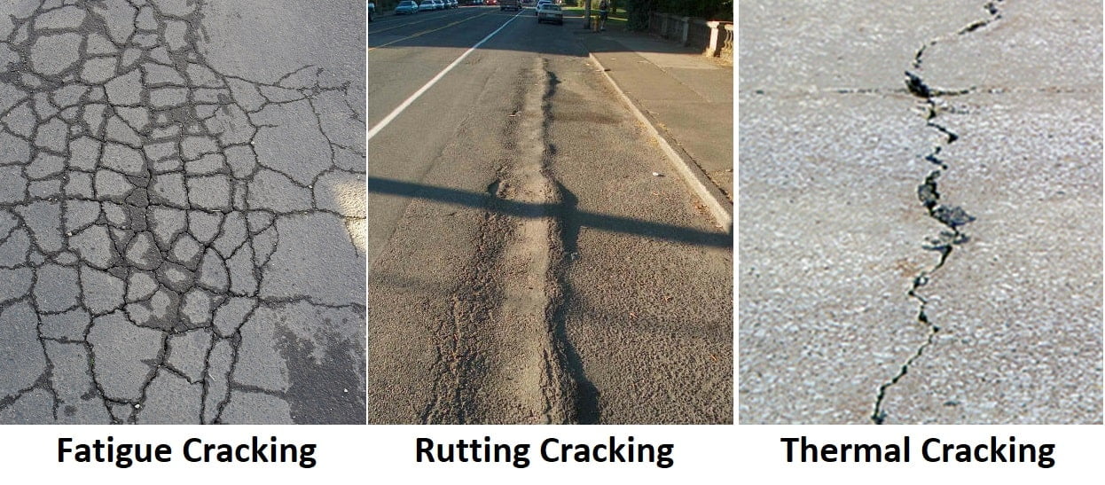
6. Major pavement failure are Fatigue cracking, Rutting & thermal Cracking. (IRC considers only fatigue cracking and rutting for flexible pavement design.)
7. A typical flexible pavement consist of four components – Surface course, Base course, Sub base course, Soil subgrade.

Note:

• Rutting is the depression in localized area.
• Thickness is always calculated above the subgrade value.

Rigid Pavement

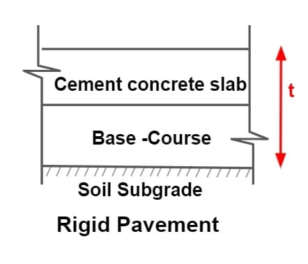
1. A rigid pavement is constructed with cement concrete slabs.
2. A rigid pavement depends upon the flexural strength or beam action of the slab for with standing the wheel load. Thus, a major contributor to the load bearing capacity is the slab itself.
3. Rigid pavement layer does not reflect the deformation of the lower layer due to the presence of concrete slab at the top.
4. Here the transfer of load takes place by the layer to layer contact.
5. Major pavement failure are fatigue cracking and pumping. (IRC considers only fatigue cracking failure for its design.)
6. Expansion & contraction joints ate required in rigid pavement.
7. A typical rigid  pavement consist of three components – Cement concrete slab, Base course, Soil Sub-grade.

Note: Pumping is the ejection of soil slurry through joints and cracks of cement concrete pavement causing downward movement of slab under heavy load.

Semi Rigid Pavement

1. A Semi-rigid pavement represents the intermediate stage between the flexible and the rigid types.
2. It derives the strength by both load spreading and flexural action.

Composite Pavement

• A composite pavements has a mixture of the above types in its layers.
• For example pavement consisting of lean concrete base, a roller compacted concrete slab over it and a surfacing of bituminous concrete.

  Difference Between Flexible and Rigid Pavement  

	Flexible Pavement	Rigid Pavement
Flexural Strength	Very low	High
No of layers	4 (Surface course, Base course, Sub base course, Soil subgrade)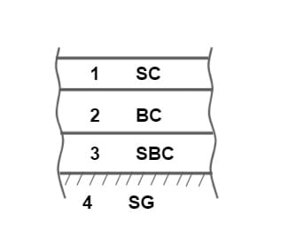	3 (Cement concrete slab, Base course, Soil subgrade)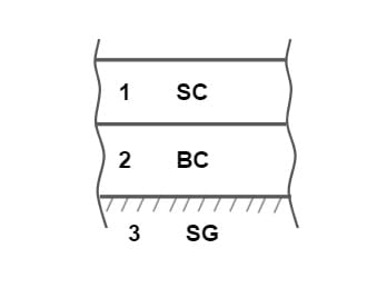
Load transformation	It is through grain to grain contact.	It is through layer to layer.
Failure	If there is any failure at the bottom then failure is appeared to the top.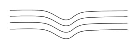	If there is any failure at the bottom then the slab will act as a bridge over the small cavity.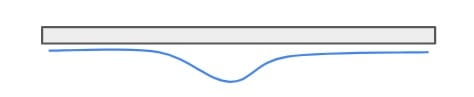
Joints	No joints required.	Expansion & contraction joints are provide.
Cost	Low initial cost and High maintenance cost.	High initial cost and Low maintenance cost.

  Functions of Pavement Components  

Soil Subgrade

• The pavement load is ultimately taken by soil subgrade.
• It is a layer of natural soil prepared to receive stress from layer above.
• Top 50 cm layer of soil subgrade is compacted properly.

Sub Base and Base Course

• These layers are composed of broken stone aggregates of smaller size.
• Base and sub base courses are used under flexible pavement for load carrying capacity by the
• distribution.
• Base course is provided under rigid pavement for preventing pumping & protecting the sub grade against frost action.

Wearing course

• Purpose of this course is to give smooth riding surface to the vehicles.
• It resists pressure exerted by vehicles and is subjected to wear and tear.
• It makes the pavement watertight.

---

  Design Parameters of  Pavement  

Standard Axle Load

The design axle load in many countries, including India is 80 kN.

So max standard axle load= 8170kg = 8.2T =80 KN

Rigidity Factor(RF)

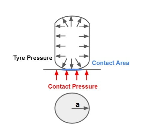
RF = \(\frac{\text{Contact Pressure}}{\text{Tyre Pressure}}\).

\(\frac{\text{CP}}{\text{TP}}\)

For Design, CP = TP = 7Kg/cm²

Tyre Pressure(Kg/cm²)	R.F
TP > 7Kg/cm²	R.F<1
TP = 7Kg/cm²	R.F=1
TP < 7Kg/cm²	R.F>1

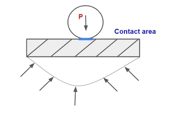
Contact Pressure and Tyre Pressure

Pressure generated at the point of contact between tyre and pavement is termed as “Contact Pressure” where as pressure inside the tyre is termed as “Tyre Pressure”.

For Design Tyre Pressure = 7 Kg/cm²

Contact Pressure = \(\frac{\text{Wheel Load }}{\text{Contact Area}}\).

Note:

If contact area is assume to be circular then A=πa².

At low tyre pressure, tyre come under compression and CP is greater then TP.

At high tyre pressure, tyre come under tension and CP is less then TP.

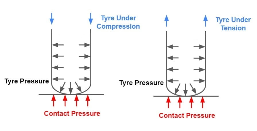
Tyre pressure is a important for upper layer while contact pressure is important for bottom layers.

Equivalent Single Wheel Load (ESWL for dual wheel Assembly)

It is defined as the load on single tyre which will cause an equal magnitude of parameter such a stress- strain and deflection to the given location to that resulting from multiple wheel load at the same location.

It is based on following assumptions.

• Equalancy concept is based on equal stress.
• Contact area is circular.
• Influence angle is 45°.
• Soil medium is elastic, homogenous and isotropic.

In a dual wheel load assembly, let ‘d’ is the clear gap between two wheel, ‘S’ be the spacing between center of the wheels and ‘a’ be the radius of the circular contact area of each wheel.

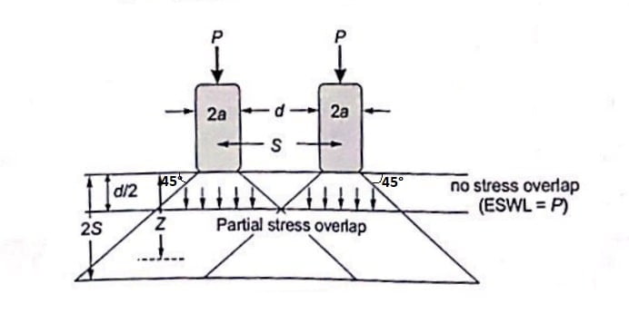
Therefor (S=d+2a)

Where, P= Wheel load, Z= Desired depth.

For

z ≤ d/2	ESWL= P (as there is no stress overlap)
z ≥ d/2	ESWL= 2S (Full overlap of stress is considered)
d/2 < z < 2S	ESWL is computed by interpolation considering the variation of ESWL to be linear with depth on log scale.

The ESWL is given by:

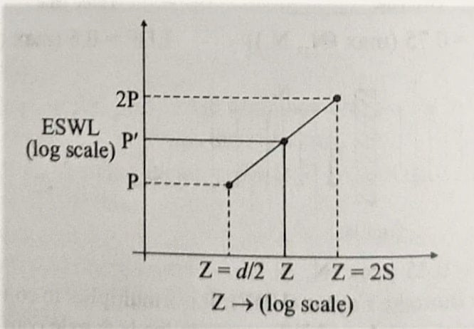
\(log P’ =log P+ \left [ \frac{log 2P-log P }{log 2S-log (d/2)} \right ]\times \left [ log Z-log (d/2) \right ]\).

---

 Example.1   what is the equivalent single wheel load of dual wheel assembly carrying 21,000 N each form pavement thickness of 20cm? Centre to centre  spacing of tyres is 28 cm and the distance between the walls of tyres is 10 cm.

Solution 

Given

S=28 cm,

d= 10cm,

P=21000 N

ESWL at d/2 depth i.e at 5 cm = 21000 N

ESWL at 2S depth i.e at 56 cm = 2×21000= 42000 N

log P’ =log 21000+ \left [ \frac{log 42000-log 21000 }{log 56-log 5} \right ]\times \left [ log 20-log 5 \right ]

log P’ = 4.49495

P’= 31257.60N

---

  No of Repetition  

As per IRC: 37-1980, flexible pavement should be designed for a cumulative no of standard axial load repetitions, throughout the design life of road, instead of designing in terms of commercial vehicle per day.

As per IRC, thickness of pavement depends on

• Severe value of subgrade
• Cumulative no of standard axle load repetitions (Ns)

Numerically

Cumulative no of standard axle load (Ns) Repetitions throughout the design life of road is calculated as:

\(Ns= \left ( \frac{365A\times D\times F\left [ (1+r)^{n}-1 \right ]}{r} \times LSF \right )_{CSA}\)

CSA→ Cumulative no of standard Axle, MSA→ Millions of standard Axle. (1MSA = 1×10⁶ CSA )

A= initial traffic in the year of completion of construction in terms of commercial vehicle per day.

D= Lane distribution factor (lateral distribution factor)

F= vehicle damage factor

r= rate of growth of traffic

n= design life of road

LSF= load safety factor (it is factor of safety, if not given then considered 1).

Note

A

A= initial traffic in the year of completion of construction in terms of commercial vehicle per day (CVPD).

1. Any vehicle which has gross weight minimum 3 tones considered as commercial vehicle.
2. If present traffic volume is ‘P’ then traffic after x years of construction period will be A=P(1+r)ⁿ.
3. A is always taken total traffic per carriageway.
   1. For single carriageway road. A should be taken at sum of both direction traffic.
   2.  For dual carriageway road. A should be taken at sum of one direction traffic.

Lane Distribution Factor (L.D.F)

it is represented by ‘D’.

According to IRC: 37-2018, lane distribution factor are as follows:

Single Carriageway

IRC: 37-2018

Single lane	D= 1(N1+N2)
Two lane	D= 0.50(N1+N2)
Four lane	D= 0.40(N1+N2)

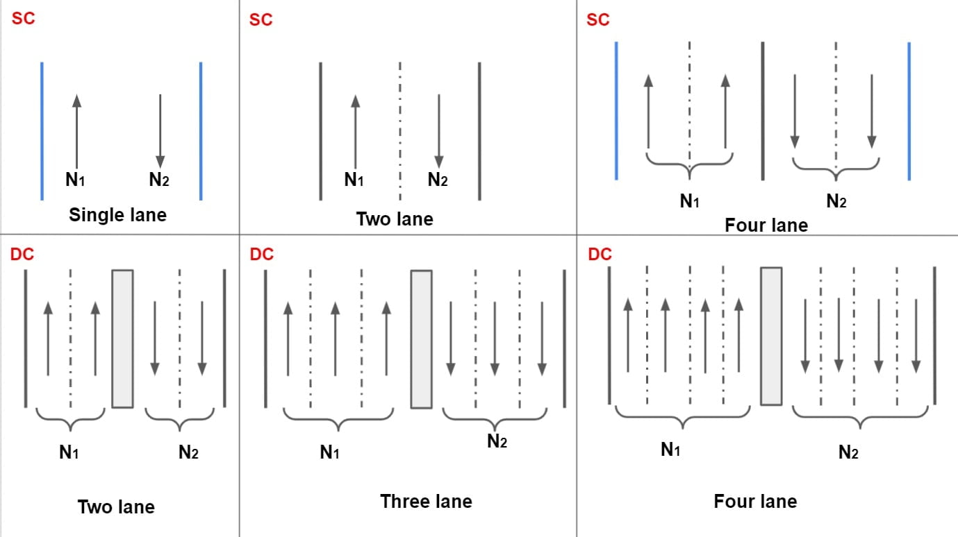
Dual Carriageway

Two lane	D= 0.75(max (N1 , N2))
Three lane	D= 0.6(max (N1 , N2))
Four lane	D= 0.45(max (N1 , N2))

Vehicle Damage Factor 

⇒ It is equivalent to no of standard axle per commercial vehicle. it is represented by ‘F’.

⇒ It is a factor which converts no of commercial vehicle of different axle load to the no of standard axle load repetitions.

⇒ It is calculate by 4th power law.

EALF ⇒ \((\frac{L_o}{L_s})^{4}\)

L_o = other axle load

L_s = standard axle load

⇒  If  L₁ axle load has percentage frequency f₁ and

L₂ axle load has percentage frequency f₂ —–

so on—–

L_n axle load has percentage frequency f_n .

Vehicle damage factor would be

F=\(\frac{f_1}{100}(\frac{L_1}{L_s})^{4}+\frac{f_2}{100}(\frac{L_2}{L_s})^{4}—+\frac{f_n}{100}(\frac{L_n}{L_s})^{4}\)

Equivalent axle load Factor (EALF)

The damage caused to the pavement by one application of the axle load under consideration relative to the damage caused by single application of standard axle load of 80 KN. In this, design is governed by No. of repetations of standard axle.

EALF of a axle load = \(\left (\frac{\text{axle load}}{\text{standard axle load}} \right )^{4}\).

Eg; 160kn axle load has EALF = \(\left (\frac{160}{80} \right )^{4}=16\).

---

 Example.2   If the standard axle load is 80KN then find out the equivalent daily number of repetition for the following data:

Axle (KN)	Repetition
35-45	800
75-85	400

Solution 

\(L_1=\frac{35+45}{2}=40KN\), N₁ = 800

\(L_2=\frac{75+85}{2}=80KN\), N₁ = 400

N = \(800\times \left ( \frac{40}{80} \right )^{4}+400\times \left ( \frac{80}{80} \right )^{4}\).

N= 450.

---

 Example.3   It is proposed to widen and strengthen existing two lane national highway section as a divided highway. find out the number of standard axle load if the existing traffic in one direction is 2500 commercial vehicle per day construction will take one year, r=8%, vehicle damage factor= 3.5% lane distribution factor = 0.75 and design life of 10 years .

Solution 

r=8%

F= 3.5

D= 0.75

x= 1years

n=10years

P= 2500CVPD

∴A= P(1+r)^x

A=\(2500\left ( 1+\frac{8}{100} \right )^{1}\)

A=2700CVPD

\(Ns= \left ( \frac{365\times A\times D\times F\left [ (1+r)^{n}-1 \right ]}{r} \times LSF \right )_{CSA}\).

\(Ns= \left ( \frac{365\times 2700\times 0.75\times 3.5\left [ (1+0.08)^{10}-1 \right ]}{0.08\times 10^{6}} \times 1 \right )_{MSA}\)

Ns=37.47 MSA

---

 Example.4   Number of commercial vehicle per day when construction is completed = 5640, design life = 20years, rate of growth of traffic= 7.5%, load safety factor=1.3, lane distribution factor=0.75, find out design traffic in ‘MSA’ for the following data:

Axle (tonne)	frequency (%)
18	10
14	20
10	35
8	15
6	20

Solution 

\(Ns= \frac{f_1}{100}\left ( \frac{L_1}{L_s} \right )^{4}+\frac{f_2}{100}\left ( \frac{L_2}{L_s} \right )^{4}+ …+\frac{f_5}{100}\left ( \frac{L_5}{L_s} \right )^{4}\).

\(Ns= \frac{10}{100}\left ( \frac{18}{8.2} \right )^{4}+\frac{20}{100}\left ( \frac{14}{8.2} \right )^{4}\)+\(\frac{35}{100}\left ( \frac{10}{8.2} \right )^{4}+\frac{15}{100}\left ( \frac{8}{8.2} \right )^{4}\)+\(\frac{20}{100}\left ( \frac{6}{8.2} \right )^{4}\).

Ns= 4.988

\(Ns= \left ( \frac{365\times 5640\times 0.75\times 4.988\left [ (1+0.075)^{20}-1 \right ]}{0.075\times 10^{6}} \times 1.3 \right )_{MSA}\)

Ns= 433.54MSA

---

  Method of Pavement Design  

Various approach for flexible pavement design may be classified in a three  groups.

Empirical Method

• These are based on physical properties and strength parameter of soil subgrade.
• Group index method, CBR method, Stabilometer method and Mc-lead method etc. are empirical methods.

Semi Empirical or Semitheoretical Method

• These methods are based on stress strain function and experience. e.g., Triaxial test method.

Theoretical Methods

These are based on mathematical computation for e.g., Burmister Method

---

  Group Index Method  

⇒ This method is based on Index properties of soil, i.e the properties which helps in identification and classification of soil.

⇒ In this method a characteristics ‘Group Index’ is used to indicate the performance of soil when used as pavement material.

⇒ G.I value lies between 0 to 20. 

⇒ Higher the G.I value poorer the soil, hence higher thickness of pavement required.

GI is given by:-

GI = 0.2a + 0.005ac + 0.0bd

where

a =(p-35) ≤ 40 [0-40]

b =(p-15) ≤ 40 [0-40]

p= % finer i.e % of partical passing through 75μ sieve.

c =(w_L-40) ≤ 20 [0-20]

w_L = liquid limit

d =(I_p-10) ≤ 20 [0-20]

I_p = plasticity Index (w_L-w_p)

⇒ To design the pavement thickness by this method first GI of soil is found.

G.I	SG Soil
0-1	Good
2-4	Fair
5-9	Poor
10-20	Very Poor

⇒ The anticipated traffic is estimated and is designated as follows

Traffic Volume	No of vehicle /day
Light	<50
Medium	50-300
Heavy	>300

⇒ Based on the anticipated traffic and group index value, thickness of pavement layer is found.

Surface Base	GI + Traffic
Subbase	GI
Subgrade

⇒ The thickness of ‘SUBBASE’ depends on only GI but thickness of ‘Base and Surface’ course is dependent on both GI & traffic.

⇒ Value of thickness of different layers of pavement is directly read from either curve or table. 

Limitations:-

This method does not consider quality of material used for pavement construction hence thickness of pavement come out to be same for poor & good quality material.

 Example.   A soil subgrade sample collected from site was analyzed of the results obtained are as follows:

• Soil proportion passing 0.075mm sieve = 60%
• w_L = 45%
• w_p=23 %

Determine the GI of subgrade & design pavement thickness using GI. Use the following data: 

GI value	Total thickness required  (cm)
0	22
5	35
10	43
15	48
20	52

Solution

a =(p-35)= 60-35= 25

b =(p-15) =60-15=45>40.

b= 40

c =(w_L-40)= 45-40=5

d =(I_p-10) = w_L-w_p -10= 45-23-10=12

GI = 0.2a + 0.005ac + 0.01bd

GI = 10.425

\(\frac{15-10}{15-10.425}=\frac{48-43}{48-t}\)

t=43.425cm

Wearing course + base course + subbase course = 43.425cm

---

  California Bearing Ratio Method (CBR Method) 

It is based on strength parameter of subgrade soil & subsequent pavement material.

Pavement thickness, t = \(\sqrt{\left ( \frac{1.75P}{CBR%} \right )-\left ( \frac{A}{\pi } \right )}\)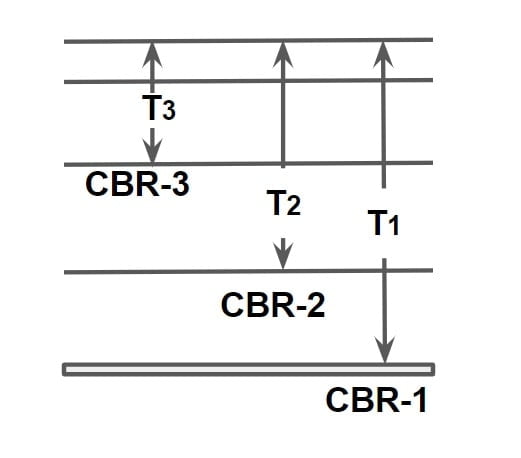

Applicable only when CBR value of CBR<12%

t= thickness in cm

CBR= in percentage

P= wheel load in kg

A= area of contact in cm²

A= π r²

r= radius of contact area.

p =P/A

A=P/p

where, p = pressure in kg/cm²

Limitations

• Quality of pavement materials in not considered.
• This method is not valid for CBR greater than 12%.

CBR value = \(\begin{Bmatrix}CBR_{2.5}= \left ( \frac{P_{2.5}}{1370} \times 100\right )\\CBR_{5.0}= \left ( \frac{P_{5.0}}{2055} \times 100\right )\end{Bmatrix}_{max}\)

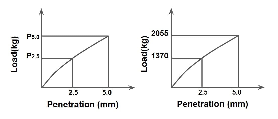
 Example.   CBR test was conducted over soil subgrade and following result were obtained.

penetration(mm)	2.5	5.0
Load(kg)	60	82

Following materials are required to be used over the soil subgrade.

• Compact soil (CBR=6%)
• Poorly graded gravel (CBR= 12%)
• Well graded gravel (CBR=60%)
• Bituminous surface (Thickness =4cm)

Design the pavement using CBR, if wheel load is 4100 kg and tyre pressure is 7 kg/cm^2. 

Solution

CBR value = \(\begin{Bmatrix}CBR_{2.5}= \left ( \frac{60}{1370} \times 100\right )\\CBR_{5.0}= \left ( \frac{82}{2055} \times 100\right )\end{Bmatrix}_{max}\).

{CBR_2.5= 4.379% and CBR₅= 3.99%} _max

so, CBR value = 4.379% =4.38%

Step.1 Thickness required S.G

\(T_1=\sqrt{\frac{1.75P}{CBR%}-\frac{P}{\pi p}}\).

\(T_1=\sqrt{\frac{1.75\times 4100}{4.38}-\frac{4100}{\pi\times 7}}\).

T₁ = 38.10cm

Step.2 Thickness required C.G

\(T_2=\sqrt{\frac{1.75\times 4100}{6}-\frac{4100}{\pi\times 7}}\).

T₂ = 31.77cm

Step.3 Thickness of pavement above PGG

\(T_3=\sqrt{\frac{1.75\times 4100}{12}-\frac{4100}{\pi\times 7}}\).

T₃ = 20.28cm

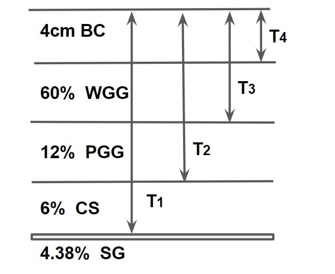
Thickness of layer:

T_CS = T₁-T₂ = 38.10-31.77 = 6.33cm

T_PGG = T₂-T₃ = 31.77-20.28 = 11.49cm

T_WGG = T₃ –T₄=  20.28-4 = 16.28cm

T_SC = 4cm

 

---

  Triaxial Test Method  

⇒ The pavement thickness T consisting of material with modulus Es is given by

\(T=\sqrt{\left ( \frac{3PXY}{2\pi E_s\Delta } \right )^{2}-a^{2}}\)

where

T= pavement thickness in cm

P= wheel load in Kg

Es = modulus of elasticity of subgrade from triaxial test result in kg/cm²

a= radius of contact area in cm 

Δ= design deflection (taken equal to 0.25 cm)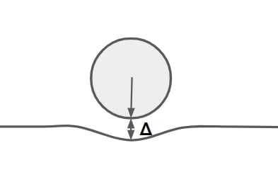

X= traffic coefficient

Y = saturation coefficient (Rainfall coefficient)

⇒ If pavement and subgrade are considered as a two layer system a ‘Stiffness factor’ has to be introduced to take into account the quality of pavement material in terms of it modulus of elasticity.

In such case thickness is given by

\(T=\sqrt{\left ( \frac{3PXY}{2\pi E_s\Delta } \right )^{2}-a^{2}}\times \left [ \left ( \frac{E_s}{E_p} \right )^{1/3} \right ]\)

E_p= modulus of elasticity of pavement 

Note: The relation between pavement layers of thickness t1 & t2 of modulus of elasticity E1 & E2 is given by 

\(\frac{t_1}{t_2}=\left ( \frac{E_2}{E_1} \right )^{1/3}\)

 Example.   Design the pavement section by triaxial test method using the following data: 

• Wheel load= 4100 kg
• Radius of contact area= 15 cm
• Traffic coefficient X= 1.5
• Rainfall coefficient Y= 0.9
• Design deflection Δ= 0.25cm
• E value of subgrade soil E_s = 100 kg/cm²
• E value of base course materials E_b =400 kg/cm²
• E value of 7.5 thick bituminous concrete surface course materials  =1000 kg/cm^2\

Solution:

Assuming the pavement to consist of single layer of base course material only, the pavement thickness is given by

\(T=\sqrt{\left ( \frac{3PXY}{2\pi E_s\Delta } \right )^{2}-a^{2}}\times \left [ \left ( \frac{E_s}{E_p} \right )^{1/3} \right ]\).

\(T=\sqrt{\left ( \frac{3\times 4100\times 1.5\times 0.9}{2\pi \times 100\times 0.25 } \right )^{2}-15^{2}}\times \left [ \left ( \frac{100}{400} \right )^{1/3} \right ]\).

T= 65.9 cm

Let, 7.5 cm bituminous concrete surface with E_c = 1000 kg/cm² be equivalent to the thickness t_b of base course. The equivalent replacement t_b, is obtained from the relation

\(\frac{t_b}{t_c}=\left ( \frac{E_c}{E_b} \right )^{1/3}\).

\( t_b =7.5\times \left ( \frac{1000}{400} \right )^{1/3}\).

t_b= 10.2cm

∴The required base course thickness 65.9-10.2=55.7 cm

The pavement section consists of 55.7 cm thick WBM base course and 7.5 cm thick bituminous concrete surface course.

---

  Design of Rigid Pavement  

⇒ It is constructed using cement concrete and its load carrying capacity is primarily due to rigidity of slab.

⇒ Rigidity is due to high modulus of elasticity of concrete.

⇒ Cement concrete pavement is rested on soil foundation which can be treated as a spring having spring constant ‘K’.

⇒ This ‘K’ is termed as ‘Modulus of Subgrade Reaction’.

Modulus of Subgrade Reaction

⇒ It is defined as load or pressure required to attain standard settlement (0.125 cm) and is found using plate load test.

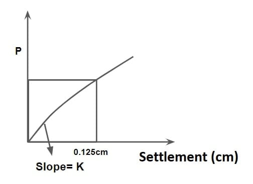
\(K= \frac{p }{\Delta }\)

\(K= \frac{p }{0.125}\)

where 

p = tyre pressure or contact pressure (kg/cm²)

Δ= deflection= 0.125cm

K = Modulus of Subgrade Reaction(kg/cm³)

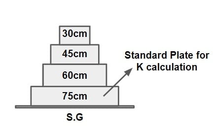
⇒To perform plate load test, different size of plate are available75cm, 60cm, 45cm, 30cm.

⇒ However IRC recommends use of 75 cm plate for this test.

⇒ As per IRC, the modulus subgrade reaction corresponding to 75 cm plate used for testing is 1/2 of that using 30cm plate.

K_75cm=0.5K₃₀

Note

For plate load test \(\Delta = \frac{1.18pa}{E_s}\). –(1)

\(\Delta = \frac{p}{K}\). –(2)

From 1 &2

\(\frac{1.18pa}{E_s} = \frac{p}{K}\)

\(Ka = \frac{E_s}{1.18}\)

Ka = constant

K₁a₁= K₂a₂

where 

p = tyre pressure or contact pressure (kg/cm²)

Δ= deflection

K = Modulus of Subgrade Reaction(kg/cm³)

E_s = Modulus of elasticity of subgrade

 Example.   A plate bearing test was carried out on a subgrade using a 76 cm diameter rigid plate. A deflection of 1.25mm was caused by a pressure of 0.84kg/cm². The modulus of subgrade reaction in kg/cm³ is

Solution 

Δ=1.25mm

p=0.84 kg/cm²

modulus of subgrade reaction for 76 cm diameter rigid plate

K₁ = p/Δ = 0.84/0.125 =6.72kg/cm₃

∴ Modulus of subgrade reaction for standard plate of radius 75cm

K₁ a₁=K a

K= K₁ a₁ /a= (6.72× 76)÷75= 6.81 kg/cm³

Radius of Relation Stiffness (l)

⇒ It is a radius of area of soil effective in resisting the deformation of slap or  pavement.

\(l=\left ( \frac{Eh^{3}}{12K(1-\mu ^{2})} \right )^{1/4}\)

E= modulus of elasticity of cement concrete in Kg/cm² (3×10⁵ Kg/cm³)

K= modulus of subgrade reaction

h= slab thickness in cm

μ= concrete poisson ratio= 0.15

l=Radius of Relation Stiffness (cm)

 Example.   Compute the radius of relative stiffness of 20 cm thick cement concrete slab from the following data:

• Modulus of elasticity of cement concrete = 2.1×10⁵ kg/cm².
• poisson ratio for concrete = 0.15
• load sustained by rigid plate= 200kg

Solution 

let diameter of plate used = 75cm

contact area of rigid plate = π (75/2)² = 4417.86cm²

pressure sustained by 75 cm = load/ contact area = 2000/4417.85 =0.453kg/cm²

Now modulus of subgrade reaction

K= p/Δ = 0.453/0.125 = 3.62kg/cm³

therefore relative stiffness of slab to subgrade

\(l=\left ( \frac{Eh^{3}}{12K(1-\mu ^{2})} \right )^{1/4}\).

\(l=\left ( \frac{2.1\times 10^{5}\times 20^{3}}{12\times 3.62(1-0.15^{2})} \right )^{1/4}\).

l=79.31cm

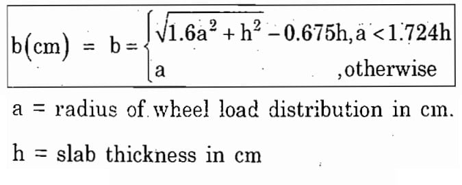
Equivalent Radius of Relation Section 

⇒  Only a small area of pavement is resisting a bending movement of a plate due to loading.

⇒  The radius of this area is termed as equivalent radius of resisting section and is given by WESTER GARD’S.

 Example.   Find the equivalent radius of resisting section of 20cm slab. if the contact area is 707cm².

Solution 

h=20cm

A=707cm² =πa²

a=15cm

\(\frac{a}{h}=\frac{15}{20}=0.75< 1.72\)

therefore \(b=\sqrt{1.6a^{2}+h^{2}}-0.675h\).

\(b=\sqrt{1.6\times 15^{2}+20^{2}}-0.675\times 20\).

b= 14.07cm

---

  Factors Affecting Pavement Design  

The structural design of rigid pavements is governed by a number of factors, such as:

(1) Loading

1. Wheel load and its repetition
2. Area of contact of wheel
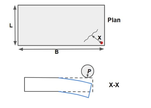
3. Location of load with respect to slab

(ii) Properties of subgrade

1. Subgrade strength and properties
2. Sub-base provision

(iii) Properties of concrete

1. Strength
2. Modulus of elasticity
3. Poisson’s ratio
4. Shrinkage properties
5. Fatigue

(iv) External conditions

• Temperature changes
• Friction between slab and subgrade

(v) Joints

• Arrangements of joints
• Spacing of joints

(vi) Reinforcement

• Quantity of reinforcement
• Continuous reinforcement

---

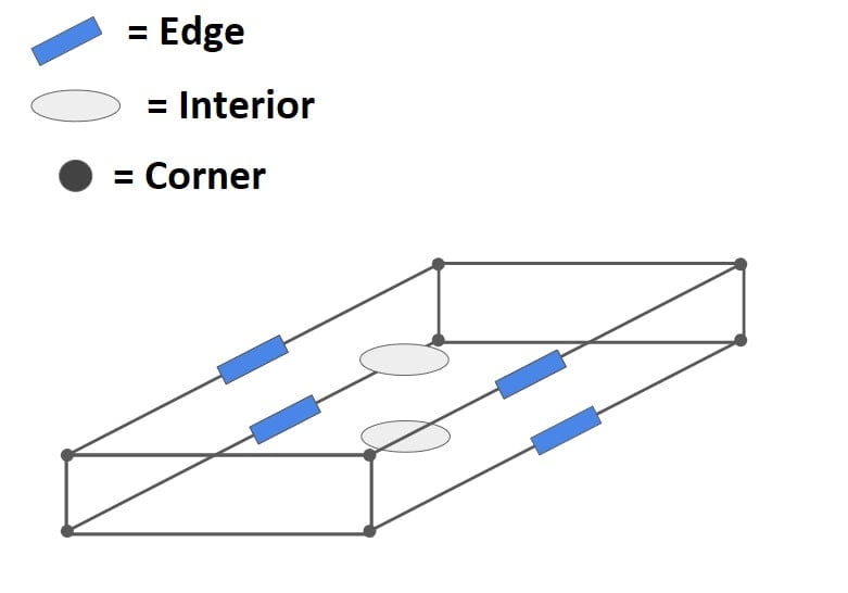
  Analysis of Stress  

Critical locations for development of stresses are as follows:

• Interior of slab
• Edge of slab
• Corner  of slab

Note: Interior of slab, Edge of slab, Corner  of slab at both top & bottom of slab.

Load Stress

⇒ This stress develops  in longitudinal direction of the slab due to wheel load.

⇒ In can be computed using WESTERGARDS theory as follows in Kg/cm².

⇒ For Interior Region

\(S_{Li}=\frac{0.316P}{h^{2}}[4log_{10}(l/b)+1.069]\)

⇒ For Edge Region

\(S_{Le}=\frac{0.572P}{h^{2}}[4log_{10}(l/b)+0.359]\)

⇒ At Corner Region

\(S_{Lc}=\frac{3P}{h^{2}}\left [1-\left ( \frac{a\sqrt{2}}{l} \right)^{0.6} \right ]\)

P= wheel load (kg)

h= thickness of slab(cm)

l= radius of relative stiffness(cm)

b= radius of equivalent resisting section (cm)

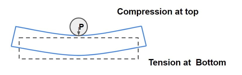
Nature of there stress are as follows:

(A) At Interior/ Edge Region

(B) At Corner  of slab

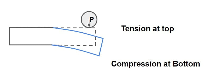
Note: Position of crack due to corner loading is given by \(x= 2.58\sqrt{al}\)

a= radius of contact area(cm)

l= radius of relative stiffness(cm)

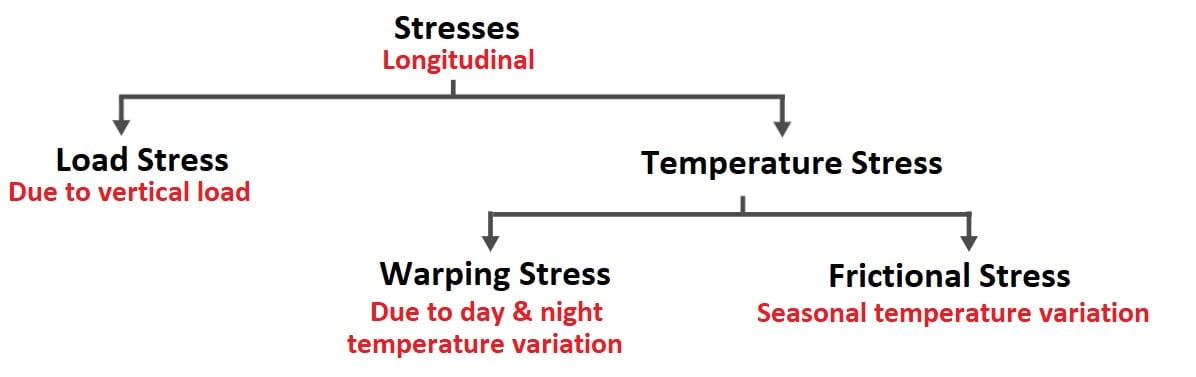
Temperature Stresses

⇒These are developed in cement concrete pavement due to variation in the slab temperature and resistance against deformation by the weight of slab & friction between slab & ground surface.

⇒ These stresses are caused by:

• Daily variation of temperature
• Seasonal variation of temperature

These stresses are of two types.

1. Warping Stress
2. Frictional Stress

Warping Stress 

⇒ This stress develops in longitudinal direction of slab due to day night temperature  variation.

⇒ Due to day night temperature variation, temperature gradient exist in top and bottom of slab. (Due to temperature gradient, it bends.)

⇒ During day time temperature at top is greater than bottom hence slab tries to expand at top & contract at the bottom which is resisted by weight of slab that result in development of compressive stress at top & tensile stress at bottom of slab.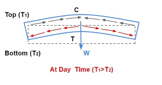

⇒ During night time temperature at top is less than bottom hence slab tries to contract at top & expand at the bottom which is resisted by weight of slab that result in development of tensile stress at top & compressive stress at bottom of slab.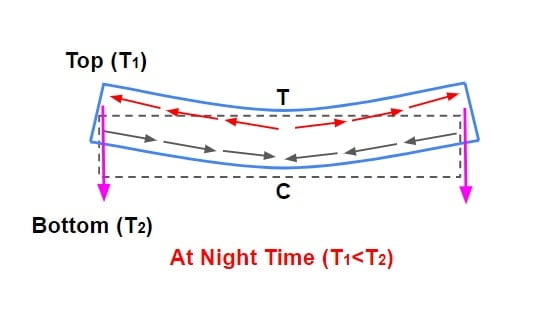

Note:

• If the slab is assumed to be weightless then there is no warping stress as there is no resistance to deformation due to temperature variation.
• Maximum warping stress will be developed at centre location.

The magnitude of these stresses are as follows:

At Interior Side

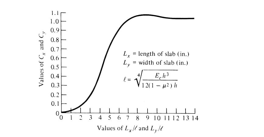
\(St_i=\frac{E\alpha t}{2}\left ( \frac{C_x+\mu C_y}{1-\mu ^{2}} \right )\)

At Edge Side

\(St_e=max\left \{ \frac{C_xE\alpha t}{2}\text{ or }\frac{C_yE\alpha t}{2}\right \}\)

At Corner Side

\(St_c=\frac{E\alpha t}{3(1-\mu )}\sqrt{\frac{a}{l}}\)

Where

E= modulus of elasticity of concrete (3×10⁵ kg/cm³)

α= coefficient of thermal expansion of concrete

t= temperature difference between top and bottom of concrete slab

μ= concrete’s poisson ratio = 0.15

l= radius of relative stiffness (cm)

a= radius of area of contact (cm)

C_x, C_y = coefficient depending upon L_x/l , L_y/l respectively and is found graphically.

L_x = spacing between transverse joints of slab,

L_y = spacing between longitudinal joint of slab.

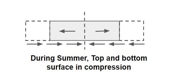
Frictional Stress

⇒ These stresses are developed due to seasonal variation of temperature & in this case there is no temperature gradient across the thickness. 

⇒ During winter, slab tries to contract due to temperature fall and the internal movement of slab is resisted by friction, which leads to the development of tensile stresses in it.

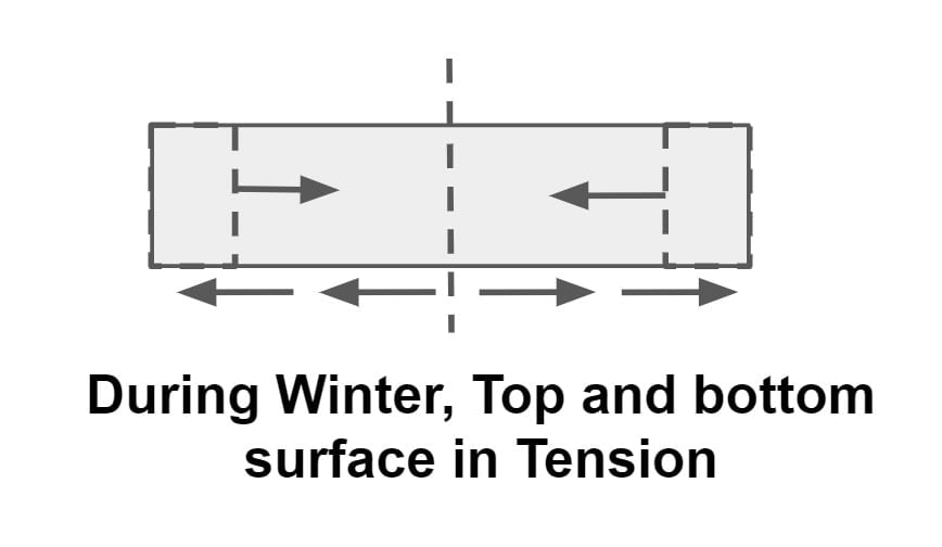
⇒ During summer, slab tries to expand due to temperature rise and the internal movement of slab is resisted by friction, which leads to the development of compressive stresses in it.

 

Stress developed in cement concrete Pavement is

\(S_f=\frac{WLf}{2\times 10^{4}}\)

Sf = unit stress developed in cement concrete pavement, kg/cm²

W= unit weight of concrete, kg/cm³ (about 2400 kg/m³)

f= coefficient of subgrade restraint (maximum value is about 1.5)

L= slab length (metre)

B= slab width, (metre)

Note:

1. Frictional stresses at corner is zero.
2. Frictional stresses is maximum at centre.
3. Generally frictional stresses are assumed to be constant along the length, but in actual it varies linearly.

  Worst Combination Of Stress 

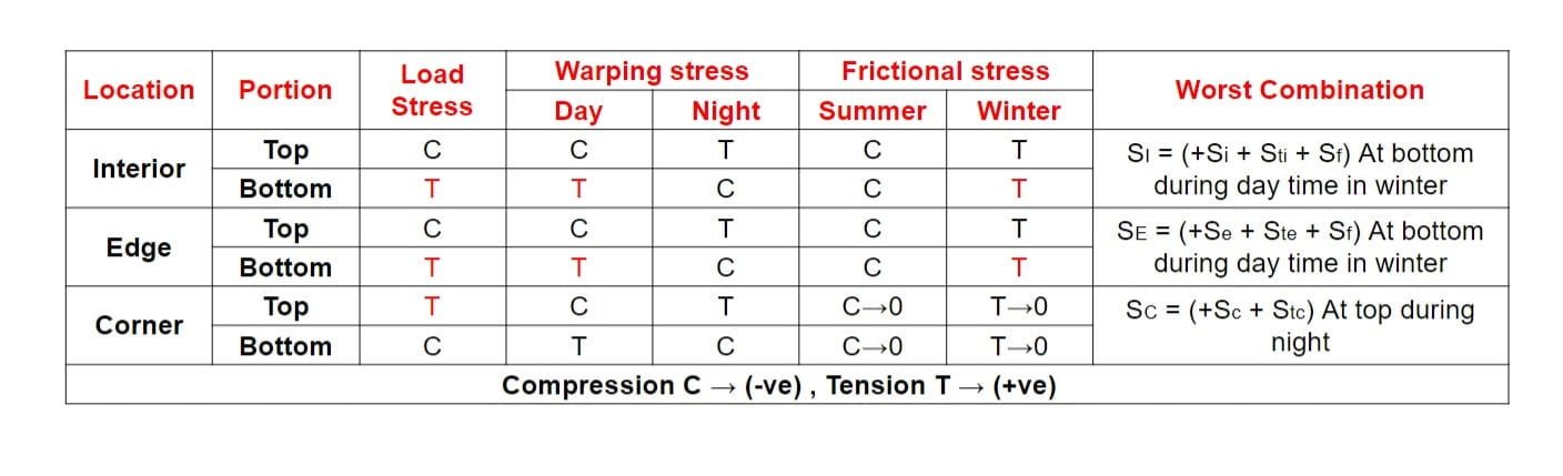
Critical Cases of Stress Combination

In combination of wheel load and temperature, edge region is most critical hence designing is done using edge region stress and however checking is done for corner region.

(i) Summer, mid- day: The critical combination of  stress for edge region is given by

S_critical = S_{load edge} + S_{warping edge} – S_friction

(ii) Winter, mid- day: The critical combination of  stress for edge region is given by

S_critical = S_{load edge} + S_{warping edge} + S_friction

(iii)Mid- night: The critical combination of  stress for corner region is given by

S_critical = S_{load corner}+ S_{warping edge}  

	Wheel Load	Temperature
Corner	Maximum	Minimum
Edge	Intermediate	Intermediate
Interior	Minimum	Maximum

 Example.   A cc pavement slab of thickness 20 cm is constructed over a granular sub base having modulus of reaction 15kg/cm³. The maximum temperature difference between the top and bottom of slab during summer day and night is found to be 18°c. The spacing between the traverse contraction joint is 4.5m and that between longitudinal joints is 3.5m. The design wheel load is 5100kg , radius of contact area is 15cm, E value for cc is 3×10⁵ kg/cm² , μ = 0.15 and α of cc = 10×10^-6 /°c and friction coefficient = 0.15 using Wester Gard’s stress equation for wheel loads at interior, edge or corner of slab and the chart for the warping stress coefficient find the worst combination of stress at the interior edge and corner.

Lx/l  or Ly/l	2	4	6	8	10	12	14
Cx or Cy	0.05	0.5	0.89	1.05	1.06	1.02	1.01

Solution 

h=20cm

K= 15kg/cm³

T= 18°c

P= 5100kg

a=15cm

E = 3×10⁵ kg/cm²

μ = 0.15

α of cc = 10×10^-6 /°c

f= 1.5

Before calcuted the value of load stress, we need the value of l, b

\(l=\left ( \frac{Eh^{3}}{12K(1-\mu ^{2})} \right )^{1/4}\).

\(l=\left ( \frac{3\times 10^{5}\times 20^{3}}{12\times 15(1-0.15^{2})} \right )^{1/4}\).

l=60.77cm

\(\frac{a}{h}=\frac{15}{20}=0.75< 1.72\).

therefore \(b=\sqrt{1.6a^{2}+h^{2}}-0.675h\).

\(b=\sqrt{1.6\times 15^{2}+20^{2}}-0.675\times 20\).

b= 14.07cm

Step.1 Load stress

\(S_{Li}=\frac{0.316P}{h^{2}}[4log_{10}(l/b)+1.069]\).
\(S_{Li}=\frac{0.316\times 5100}{20^{2}}[4log_{10}(60.77/14)+1.069] = 14.58 kg/cm^{2} \).

 

\(S_{Le}=\frac{0.572P}{h^{2}}[4log_{10}(l/b)+0.359]\).
\(S_{Le}=\frac{0.572\times 5100}{20^{2}}[4log_{10}(60.77/14)+0.359]= 21.21 kg/cm^{2}\).

 

\(S_{Lc}=\frac{3P}{h^{2}}\left [1-\left ( \frac{a\sqrt{2}}{l} \right)^{0.6} \right ]\).
\(S_{Lc}=\frac{3\times 5100}{20^{2}}\left [1-\left ( \frac{15\sqrt{2}}{60.77} \right)^{0.6} \right ]= 17kg/cm^{2}\).

 

Step.2 Warping Stress 

\(\frac{L_x}{l}=\frac{4.5}{0.6077}\) = 7.40

By interpolating (table given in question)

the value of C_x = 1

\(\frac{L_y}{l}=\frac{3.5}{0.6077}\) = 5.76

By interpolating (table given in question)

the value of C_y = 0.84

\(St_i=\frac{E\alpha t}{2}\left ( \frac{C_x+\mu C_y}{1-\mu ^{2}} \right )\).
\(St_i=\frac{3\times 10^{5}\times 10\times10^{-6}\times18}{2}\left ( \frac{1+0.15\times0.84}{1-0.15^{2}} \right )\).
\(St_i=31.10kg/cm^{2}\).

 

\(St_e=max\left \{ \frac{C_xE\alpha t}{2}\text{ or }\frac{C_yE\alpha t}{2}\right \}\).
Cx>Cy , so
\(St_e=\frac{C_xE\alpha t}{2}\).
\(St_e=\frac{1\times 3\times 10^{5}\times 10\times10^{-6}\times18}{2}\).
\(St_e=27kg/cm^{2}\).

 

\(St_c=\frac{E\alpha t}{3(1-\mu )}\sqrt{\frac{a}{l}}\).
\(St_c=\frac{3\times 10^{5}\times 10\times10^{-6}\times18}{3(1-0.15)}\sqrt{\frac{15}{60.77}}\).

\(St_c=10.52kg/cm^{2}\).

Step.3 Frictional  Stress 

\(S_f=\frac{WLf}{2\times 10^{4}}\).
\(S_f=\frac{2400\times4.5\times1.5}{2\times 10^{4}}\).

\(S_f=0.81kg/cm^{2}\).

Step.4 Worst Combination

SI = (+Si + Sti + Sf)= 14.58+31.1+0.81 = 46.49kg/cm²

SE = (+Se + Ste + Sf)= 21.21+27+0.81= 49.02kg/cm²

SC = (+Sc + Stc)= 17.9+10.52 =28.42 kg/cm²

---

---

  Design of Joints  

Different types of joints are placed in concrete pavements to limit the stresses induced by temperature changes and to facilitate proper bonding of two adjacent sections of pavement when there is a time lapse between their construction (for example, between the end of one day’s work and the beginning of the next).

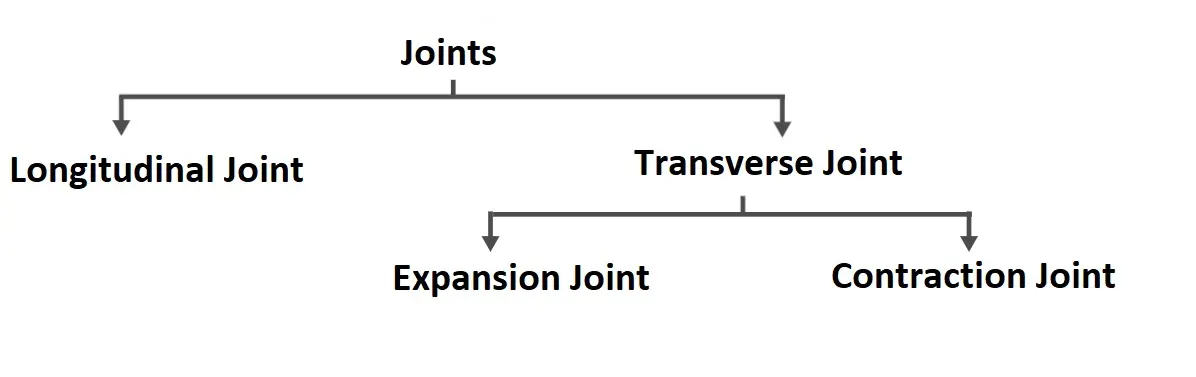
Expansion Joint

⇒ Expansion joint are provide in transverse direction to allow longitudinal expansion of slab due to increase in environment temperature with respect to construction temperature.

⇒ To design these joints we find out the joint spacing for a given joint thickness of 2.5 cm maximum as specified by IRC.

NOTE: As per IRC thickness/ width (δ) ≤ 2.5cm. And spacing (L) ≤140m.

⇒ At the expansion joint dowels are provided which develops bending, bearing & shearing stresses and help in load transfer.

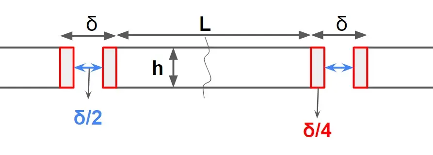
Allowable expansion  = \(\frac{\delta}{4}+\frac{\delta}{4}=\frac{\delta}{2} \)

\(\frac{\delta}{2}=L\cdot \alpha \cdot \Delta T\)

ΔT= max rise in temperature wrt construction temperature.

ΔT= T_max – T_construction

L= spacing between transverse joint

δ= width of expansion joint 

\(L=\frac{\delta}{2\cdot \alpha \cdot \Delta T}\)

Dowel Bar At expansion Joint 

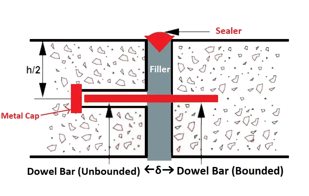
Dowel bar are provide to serve the following.

• To transfer the load from one slab to another.
• To avoid differential settlement.

As per IRC

1.  Diameter φ = 25mm
2. Length = 50 cm {20cm is bounded(40%) and  30 cm is unbounded(60%)}
3. They are positioned at centre of slab (across thickness). Depth = h/2 (h= slab thickness)
4. C/C spacing @ 300mm or less

Contraction Joint

⇒ When concrete pavement is subjected to a decrease in temperature, the slab will contract if it is free to move. Prevention of this contraction movement will induce tensile stresses in the concrete pavement. Contraction joints therefore are placed transversely at regular intervals across the width of the pavement to release some of the tensile stresses that are so induced. 

⇒ It is provided to control the irregular cracking of slab due to shrinkage & moisture variation.

⇒ Contraction joints are contracted by providing cut mark to the top of the slab.

⇒ These cut mark can also be considered as per defined crack line.

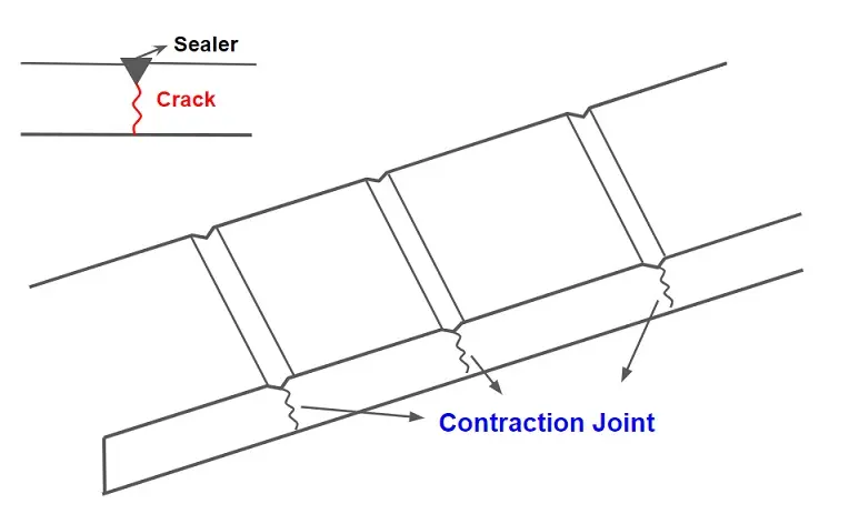
⇒ Contraction joints can be provide with or without dowel bar.

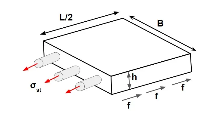
Case.1 Without Dowel Bar

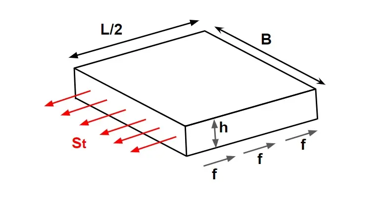
Friction force developed by half slab = Resistance force by concrete at c/s

\(f\times(\frac{L}{2}\times B \times h\times \gamma ) =S_t\times B\times h\)

\(L=\frac{2S_t}{f\gamma }\)

Where,

S_t = Tensile strength developed in concrete and is taken as 0.8 kg/cm²

γ= Unit weight of the concrete which can be taken as 2400 kg/cm³

f = Coefficient of subgrade friction which can be taken as 1.5

L= spacing b/w contraction joint

Case.2 With Dowel Bar

Friction force = force in bar

\(f\times(\frac{L}{2}\times B \times h\times \gamma ) =A_{st}\times \sigma _{st}\)

\(L =\frac{2\times A_{st}\times \sigma _{st}}{f \times B \times h\times \gamma}\)

Where,

γ= Unit weight of the concrete which can be taken as 2400 kg/m³ or 24KN/m³

f = Coefficient of subgrade friction which can be taken as 1.5

σ_st = allowable tensile stress in steel 

A_st = Total cross sectional area of steel

Note: In this case as per IRC spacing of contraction joints L≤ 4.5m.

Longitudinal Joint

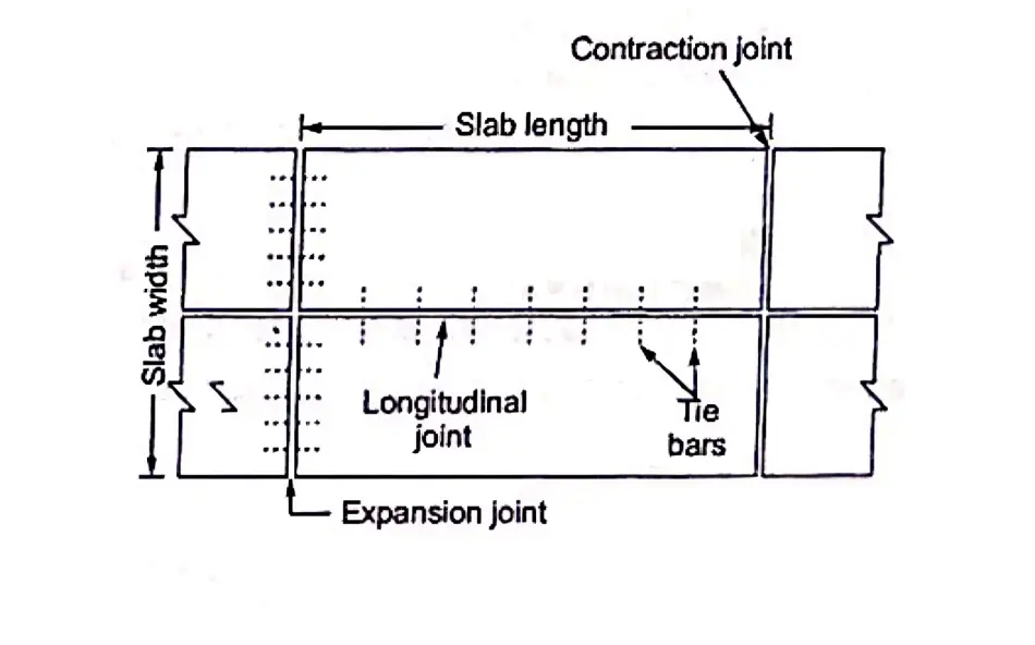
⇒ This joint is provided in longitudinal direction to allow transverse expansion and contraction of slab due to change in environment temperature.

⇒ It reduces the warping stress.

⇒The normal width of slab is generally 3-5m. If width of slab becomes more two slabs are provide along with longitudinal joint.

⇒ Tie bars are also provide at longitudinal joint.

⇒ These bars are not designed as load transfer device but ensures that the two slab remain firmly together. 

⇒ These are bounded with concrete and we mostly use deformed bars in this case.

⇒As per IRC: Diameter of the bar (φ) ≤ 20mm. And spacing (S) ≤75m.

Design of tie bars

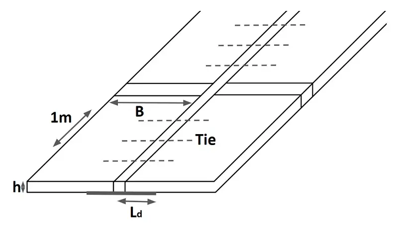
frictional force developed by 1 metre slab = Resistance force by tie bars per metre slab.

\(f\times(\gamma \times 1\times B \times h) =\sigma _{st}\times A_{st}\)/metre slab

Area of steel required per metre slab

\(A_{st}=\frac{f\times\gamma \times B \times h}{\sigma _{st}}\)

where 

B= width of pavement panel in m

h= depth of pavement in cm

γ= unit weight of concrete

σ_st = Allowable tensile stress in steel (assume 1750 kg/cm²)

f= frictional coefficient

If assume diameter of tie bars =\(\phi \)

No of  Tie bars (n) per metre slab

\(n=\frac{A_{st}}{\frac{\pi }{4}\phi ^{2}}\)

C/C spacing (S)

\(S=\frac{1000}{n}\) mm

Note: As per IRC 

• Diameter of the bar= \(\phi \) ≤ 20mm.
• Spacing = S ≤75cm.

Length of tie bars (L_t)

The length of the tie(L_t) bar is twice the length needed to develop bond stress equal to the working tensile stress and is given by:

L_t = 2 × L_d

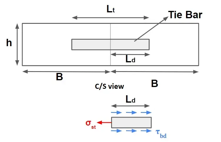
\(\sigma _{st}\times A_{st}=\tau _{bd}\times \pi \times \phi \times L_d\)

\(\sigma _{st}\times \frac{\pi \phi ^{2}}{4}=\tau _{bd}\times \pi \times \phi \times L_d\)

\(L_d=\frac{\phi\times \sigma _{st}}{4\tau _{bd}}\)

\(L_t=\frac{\phi\times \sigma _{st}}{2\tau _{bd}}\)

where 

\(\phi \)= Diameter of the bar

σ_st = Allowable tensile stress in kg/cm²

τ_bd= Allowable bond stress (=17.5 kg/cm² for plain bar and 24.6 kg/cm² for deformed bar)

---

 Example.   Calculate the spacing between contraction joints by using following data.

width of slab = 4.52m

thickness of slab = 25cm

coefficient of friction = 1.5

Allowable stress in steel = 1400kg/cm²

Dia of bar= 12mm

 Spacing between the bar = 300mm.

Solution 

A_st = n × \(\frac{\pi \times1.2^{2}}{4}\)

n= \(\frac{4.52 \times10^{3}}{300}\)= 15.06 ≅ 15

A_st = 15 × \(\frac{\pi \times1.2^{2}}{4}\)= 16.956 cm²

\(L =\frac{2\times A_{st}\times \sigma _{st}}{f \times B \times h\times \gamma}\)

\(L =\frac{2\times 16.956 cm^{2}\times 1400kg/cm^{2}}{1.5\times (2400 \times 10^{-6})Kg/cm^{3} \times(4.52 \times10^{2})cm \times25cm}\)

L= 1167.07cm = 11.67m

 Example.   If width of expansion joint is 2 cm & temperature at the time of construction of slab is 20°c, then find the spacing between expansion joint for a maximum temperature of 45°c (α=12 ×10^-6/°c)

Solution 

ΔT= 45°c-20°c= 25°c

\(L=\frac{\delta}{2\cdot \alpha \cdot \Delta T}\)

\(L=\frac{2}{2\cdot 12\times 10^{-6} \times 25}\)

L= 3333cm

L= 33.3m ≤ 140 m (safe)

 Example.   Cement concrete pavement has a thickness of 24 cm and has two lane of width 7.2m with a longitudinal joint in between. design the dimension and spacing of the bar by following data:

Allowable tensile stress in steel = 1400 kg/cm²

unit weight of cement concrete= 2400 kg/ m³

coefficient of friction =1.5

Bond stress between steel bar and concrete = 24.6kg/cm²

Solution 

\(A_{st}=\frac{f\times\gamma \times 1\times B \times h}{\sigma _{st}}\)

\(A_{st}=\frac{1.5\times 2400 \times1\times 3.6 \times24\times10^{-2}}{\frac{1400}{10^{-4}}}\)

A_st=222.14 × 10^-6 m²

A_st=222.14 mm²

Assume Dia of tie bar (\(\phi \)) = 10mm

Area of one bar = \(A=\pi \times \frac{10^{2}}{4}\) = 78.5mm²

No of bar (N)= A_st /A= 222.14 mm² /78.5mm² =3

Spacing between bar = 1000/3 = 333.33 mm = 30cm ≤ 75cm Safe

Length of tie bar \(L_t=\frac{\phi \times \sigma _{st}}{2\tau _{bd}}\)

\(L_t=\frac{10 \times 1400}{2\times 24.6}\)

L_t = 28/4.55 mm

---

  Materials Used In Rigid Pavement  

1. Portland Cement
2. Coarse Aggregates
3. Fine Aggregates
4. Water
5. Reinforcing Steel
6. Temperature Steel
7. Dowel Bars
8. Tie Bars

---

  Difference Between Dowel Bars and Tie Bars  

Dowel Bars	Tie Bars
Placed across transverse joint at the mid depth of the slab.	Placed across longitudinal joint at the mid depth of the slab.
They transfer load from slab to another without preventing the joint from opening.	They prevent lanes from separation and differential deflection.
These bars reduces joint faulting & corner cracking.	These bars reduces transverse cracking.
These bars are usually much larger in diameter than the tie bars.	These bars are usually much smaller in diameter than the dowel bars.

---

FOR MORE INFORMATION ABOUT HIGHWAY ENGINEERING